The raison d'etre of spatial databases is to perform queries inside the database which would ordinarily require desktop GIS functionality. Using PostGIS effectively requires knowing what spatial functions are available, how to use them in queries, and ensuring that appropriate indexes are in place to provide good performance.
Spatial relationships indicate how two geometries interact with one another. They are a fundamental capability for querying geometry.
According to the OpenGIS Simple Features Implementation Specification for SQL, "the basic approach to comparing two geometries is to make pair-wise tests of the intersections between the Interiors, Boundaries and Exteriors of the two geometries and to classify the relationship between the two geometries based on the entries in the resulting 'intersection' matrix."
In the theory of point-set topology, the points in a geometry embedded in 2-dimensional space are categorized into three sets:
- Boundary
The boundary of a geometry is the set of geometries of the next lower dimension. For
POINTs, which have a dimension of 0, the boundary is the empty set. The boundary of aLINESTRINGis the two endpoints. ForPOLYGONs, the boundary is the linework of the exterior and interior rings.- Interior
The interior of a geometry are those points of a geometry that are not in the boundary. For
POINTs, the interior is the point itself. The interior of aLINESTRINGis the set of points between the endpoints. ForPOLYGONs, the interior is the areal surface inside the polygon.- Exterior
The exterior of a geometry is the rest of the space in which the geometry is embedded; in other words, all points not in the interior or on the boundary of the geometry. It is a 2-dimensional non-closed surface.
The Dimensionally Extended 9-Intersection Model (DE-9IM) describes the spatial relationship between two geometries by specifying the dimensions of the 9 intersections between the above sets for each geometry. The intersection dimensions can be formally represented in a 3x3 intersection matrix.
For a geometry g
the Interior, Boundary, and Exterior
are denoted using the notation
I(g), B(g), and
E(g).
Also, dim(s) denotes the dimension of
a set s with the domain of
{0,1,2,F}:
0=> point1=> line2=> areaF=> empty set
Using this notation, the intersection matrix for two geometries a and b is:
| Interior | Boundary | Exterior | |
|---|---|---|---|
| Interior | dim( I(a) ∩ I(b) ) | dim( I(a) ∩ B(b) ) | dim( I(a) ∩ E(b) ) |
| Boundary | dim( B(a) ∩ I(b) ) | dim( B(a) ∩ B(b) ) | dim( B(a) ∩ E(b) ) |
| Exterior | dim( E(a) ∩ I(b) ) | dim( E(a) ∩ B(b) ) | dim( E(a) ∩ E(b) ) |
Visually, for two overlapping polygonal geometries, this looks like:
| ||||||||||||||||||
|
|


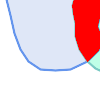
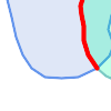

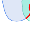
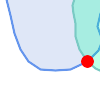
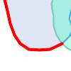
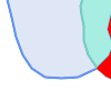
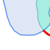

Reading from left to right and top to bottom, the intersection matrix is represented as the text string '212101212'.
For more information, refer to:
To make it easy to determine common spatial relationships, the OGC SFS defines a set of named spatial relationship predicates. PostGIS provides these as the functions ST_Contains, ST_Crosses, ST_Disjoint, ST_Equals, ST_Intersects, ST_Overlaps, ST_Touches, ST_Within. It also defines the non-standard relationship predicates ST_Covers, ST_CoveredBy, and ST_ContainsProperly.
Spatial predicates are usually used as conditions in SQL WHERE or JOIN clauses.
The named spatial predicates automatically use a spatial index if one is available,
so there is no need to use the bounding box operator && as well.
For example:
SELECT city.name, state.name, city.geom
FROM city JOIN state ON ST_Intersects(city.geom, state.geom);
For more details and illustrations, see the PostGIS Workshop.
In some cases the named spatial relationships are insufficient to provide a desired spatial filter condition.
 For example, consider a linear
dataset representing a road network. It may be required
to identify all road segments that cross
each other, not at a point, but in a line (perhaps to validate some business rule).
In this case ST_Crosses does not
provide the necessary spatial filter, since for
linear features it returns A two-step solution
would be to first compute the actual intersection
(ST_Intersection) of pairs of road lines that spatially
intersect (ST_Intersects), and then check if the intersection's
ST_GeometryType is ' Clearly, a simpler and faster solution is desirable. |
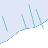 A second example is locating wharves that intersect a lake's boundary on a line and where one end of the wharf is up on shore. In other words, where a wharf is within but not completely contained by a lake, intersects the boundary of a lake on a line, and where exactly one of the wharf's endpoints is within or on the boundary of the lake. It is possible to use a combination of spatial predicates to find the required features:
|
These requirements can be met by computing the full DE-9IM intersection matrix. PostGIS provides the ST_Relate function to do this:
SELECT ST_Relate( 'LINESTRING (1 1, 5 5)',
                  'POLYGON ((3 3, 3 7, 7 7, 7 3, 3 3))' );
st_relate
-----------
1010F0212
To test a particular spatial relationship,
an intersection matrix pattern is used.
This is the matrix representation augmented with the additional symbols
{T,*}:
T=> intersection dimension is non-empty; i.e. is in{0,1,2}*=> don't care
Using intersection matrix patterns, specific spatial relationships can be evaluated in a more succinct way. The ST_Relate and the ST_RelateMatch functions can be used to test intersection matrix patterns. For the first example above, the intersection matrix pattern specifying two lines intersecting in a line is '1*1***1**':
-- Find road segments that intersect in a line
SELECT a.id
FROM roads a, roads b
WHERE a.id != b.id
      AND a.geom && b.geom
      AND ST_Relate(a.geom, b.geom, '1*1***1**');
For the second example, the intersection matrix pattern specifying a line partly inside and partly outside a polygon is '102101FF2':
-- Find wharves partly on a lake's shoreline
SELECT a.lake_id, b.wharf_id
FROM lakes a, wharfs b
WHERE a.geom && b.geom
AND ST_Relate(a.geom, b.geom, '102101FF2');When constructing queries using spatial conditions,
for best performance it is important to
ensure that a spatial index is used, if one exists (see Section 4.9, “Spatial Indexes”).
To do this, a spatial operator or index-aware function must be used
in a WHERE or ON clause of the query.
Spatial operators include the bounding box operators (of which the most commonly used is &&; see Section 7.10.1, “Bounding Box Operators” for the full list) and the distance operators used in nearest-neighbor queries (the most common being <->; see Section 7.10.2, “Distance Operators” for the full list.)
Index-aware functions automatically add a bounding box operator to the spatial condition. Index-aware functions include the named spatial relationship predicates ST_Contains, ST_ContainsProperly, ST_CoveredBy, ST_Covers, ST_Crosses, ST_Intersects, ST_Overlaps, ST_Touches, ST_Within, ST_Within, and ST_3DIntersects, and the distance predicates ST_DWithin, ST_DFullyWithin, ST_3DDFullyWithin, and ST_3DDWithin .)
Functions such as ST_Distance do not use indexes to optimize their operation. For example, the following query would be quite slow on a large table:
SELECT geom
FROM geom_table
WHERE ST_Distance( geom, 'SRID=312;POINT(100000 200000)' ) < 100
This query selects all the geometries in geom_table which are
within 100 units of the point (100000, 200000). It will be slow because
it is calculating the distance between each point in the table and the
specified point, ie. one ST_Distance() calculation
is computed for every row in the table.
The number of rows processed can be reduced substantially by using the index-aware function ST_DWithin:
SELECT geom
FROM geom_table
WHERE ST_DWithin( geom, 'SRID=312;POINT(100000 200000)', 100 )
This query selects the same geometries, but it does it in a more
efficient way.
This is enabled by ST_DWithin() using the
&& operator internally on an expanded bounding box
of the query geometry.
If there is a spatial index on geom, the query
planner will recognize that it can use the index to reduce the number of
rows scanned before calculating the distance.
The spatial index allows retrieving only records with geometries
whose bounding boxes overlap the expanded extent
and hence which might be within the required distance.
The actual distance is then computed to confirm whether to include the record in the result set.
For more information and examples see the PostGIS Workshop.
The examples in this section make use of a table
of linear roads, and a table of polygonal municipality boundaries. The
definition of the bc_roads table is:
Column    | Type              | Description
----------+-------------------+-------------------
gid       | integer           | Unique ID
name      | character varying | Road Name
geom      | geometry          | Location Geometry (Linestring)
The definition of the bc_municipality
table is:
Column   | Type              | Description
---------+-------------------+-------------------
gid      | integer           | Unique ID
code     | integer           | Unique ID
name     | character varying | City / Town Name
geom     | geometry          | Location Geometry (Polygon)
- 5.3.1. What is the total length of all roads, expressed in kilometers?
- 5.3.2. How large is the city of Prince George, in hectares?
- 5.3.3. What is the largest municipality in the province, by area?
- 5.3.4. What is the length of roads fully contained within each municipality?
- 5.3.5. Create a new table with all the roads within the city of Prince George.
- 5.3.6. What is the length in kilometers of "Douglas St" in Victoria?
- 5.3.7. What is the largest municipality polygon that has a hole?