Chapter 4. Data Management

The Open Geospatial Consortium (OGC) developed the Simple Features Access standard (SFA) to provide a model for geospatial data. It defines the fundamental spatial type of Geometry, along with operations which manipulate and transform geometry values to perform spatial analysis tasks. PostGIS implements the OGC Geometry model as the PostgreSQL data types geometry and geography.

Geometry is an abstract type. Geometry values belong to one of its concrete subtypes which represent various kinds and dimensions of geometric shapes. These include the atomic types Point, LineString, LinearRing and Polygon, and the collection types MultiPoint, MultiLineString, MultiPolygon and GeometryCollection. The Simple Features Access - Part 1: Common architecture v1.2.1 adds subtypes for the structures PolyhedralSurface, Triangle and TIN.

Geometry models shapes in the 2-dimensional Cartesian plane. The PolyhedralSurface, Triangle, and TIN types can also represent shapes in 3-dimensional space. The size and location of shapes are specified by their coordinates. Each coordinate has a X and Y ordinate value determining its location in the plane. Shapes are constructed from points or line segments, with points specified by a single coordinate, and line segments by two coordinates.

Coordinates may contain optional Z and M ordinate values. The Z ordinate is often used to represent elevation. The M ordinate contains a measure value, which may represent time or distance. If Z or M values are present in a geometry value, they must be defined for each point in the geometry. If a geometry has Z or M ordinates the coordinate dimension is 3D; if it has both Z and M the coordinate dimension is 4D.

Geometry values are associated with a spatial reference system indicating the coordinate system in which it is embedded. The spatial reference system is identified by the geometry SRID number. The units of the X and Y axes are determined by the spatial reference system. In planar reference systems the X and Y coordinates typically represent easting and northing, while in geodetic systems they represent longitude and latitude. SRID 0 represents an infinite Cartesian plane with no units assigned to its axes. See Section 4.5, “Spatial Reference Systems”.

The geometry dimension is a property of geometry types. Point types have dimension 0, linear types have dimension 1, and polygonal types have dimension 2. Collections have the dimension of the maximum element dimension.

A geometry value may be empty. Empty values contain no vertices (for atomic geometry types) or no elements (for collections).

An important property of geometry values is their spatial extent or bounding box, which the OGC model calls envelope. This is the 2 or 3-dimensional box which encloses the coordinates of a geometry. It is an efficient way to represent a geometry's extent in coordinate space and to check whether two geometries interact.

The geometry model allows evaluating topological spatial relationships as described in Section 5.1.1, “Dimensionally Extended 9-Intersection Model”. To support this the concepts of interior, boundary and exterior are defined for each geometry type. Geometries are topologically closed, so they always contain their boundary. The boundary is a geometry of dimension one less than that of the geometry itself.

The OGC geometry model defines validity rules for each geometry type. These rules ensure that geometry values represents realistic situations (e.g. it is possible to specify a polygon with a hole lying outside the shell, but this makes no sense geometrically and is thus invalid). PostGIS also allows storing and manipulating invalid geometry values. This allows detecting and fixing them if needed. See Section 4.4, “Geometrievalidierung”

POINT (1 2)
POINT Z (1 2 3)
POINT ZM (1 2 3 4)

LINESTRING (1 2, 3 4, 5 6)

LINEARRING (0 0 0, 4 0 0, 4 4 0, 0 4 0, 0 0 0)

POLYGON ((0 0 0,4 0 0,4 4 0,0 4 0,0 0 0),(1 1 0,2 1 0,2 2 0,1 2 0,1 1 0))

MULTIPOINT ( (0 0), (1 2) )

MULTILINESTRING ( (0 0,1 1,1 2), (2 3,3 2,5 4) )

MULTIPOLYGON (((1 5, 5 5, 5 1, 1 1, 1 5)), ((6 5, 9 1, 6 1, 6 5)))

GEOMETRYCOLLECTION ( POINT(2 3), LINESTRING(2 3, 3 4))

POLYHEDRALSURFACE Z (
  ((0 0 0, 0 0 1, 0 1 1, 0 1 0, 0 0 0)),
  ((0 0 0, 0 1 0, 1 1 0, 1 0 0, 0 0 0)),
  ((0 0 0, 1 0 0, 1 0 1, 0 0 1, 0 0 0)),
  ((1 1 0, 1 1 1, 1 0 1, 1 0 0, 1 1 0)),
  ((0 1 0, 0 1 1, 1 1 1, 1 1 0, 0 1 0)),
  ((0 0 1, 1 0 1, 1 1 1, 0 1 1, 0 0 1)) )

TRIANGLE ((0 0, 0 9, 9 0, 0 0))

TIN Z ( ((0 0 0, 0 0 1, 0 1 0, 0 0 0)), ((0 0 0, 0 1 0, 1 1 0, 0 0 0)) )

The ISO/IEC 13249-3 SQL Multimedia - Spatial standard (SQL/MM) extends the OGC SFA to define Geometry subtypes containing curves with circular arcs. The SQL/MM types support 3DM, 3DZ and 4D coordinates.

	Alle Gleitpunkt Vergleiche der SQL-MM Implementierung werden mit einer bestimmten Toleranz ausgeführt, zurzeit 1E-8.

CIRCULARSTRING(0 0, 1 1, 1 0)

CIRCULARSTRING(0 0, 4 0, 4 4, 0 4, 0 0)

COMPOUNDCURVE( CIRCULARSTRING(0 0, 1 1, 1 0),(1 0, 0 1))

CURVEPOLYGON(
  CIRCULARSTRING(0 0, 4 0, 4 4, 0 4, 0 0),
  (1 1, 3 3, 3 1, 1 1) )

CURVEPOLYGON(
  COMPOUNDCURVE( CIRCULARSTRING(0 0,2 0, 2 1, 2 3, 4 3),
                 (4 3, 4 5, 1 4, 0 0)),
  CIRCULARSTRING(1.7 1, 1.4 0.4, 1.6 0.4, 1.6 0.5, 1.7 1) )

MULTICURVE( (0 0, 5 5), CIRCULARSTRING(4 0, 4 4, 8 4))

MULTISURFACE(
  CURVEPOLYGON(
    CIRCULARSTRING( 0 0, 4 0, 4 4, 0 4, 0 0),
    (1 1, 3 3, 3 1, 1 1)),
  ((10 10, 14 12, 11 10, 10 10), (11 11, 11.5 11, 11 11.5, 11 11)))

The OGC SFA specification defines two formats for representing geometry values for external use: Well-Known Text (WKT) and Well-Known Binary (WKB). Both WKT and WKB include information about the type of the object and the coordinates which define it.

Well-Known Text (WKT) provides a standard textual representation of spatial data. Examples of WKT representations of spatial objects are:

Input and output of WKT is provided by the functions ST_AsText and ST_GeomFromText:

text WKT = ST_AsText(geometry);
geometry = ST_GeomFromText(text WKT, SRID);

For example, a statement to create and insert a spatial object from WKT and a SRID is:

INSERT INTO geotable ( geom, name )
  VALUES ( ST_GeomFromText('POINT(-126.4 45.32)', 312), 'A Place');

Well-Known Binary (WKB) provides a portable, full-precision representation of spatial data as binary data (arrays of bytes). Examples of the WKB representations of spatial objects are:

Input and output of WKB is provided by the functions ST_AsBinary and ST_GeomFromWKB:

bytea WKB = ST_AsBinary(geometry);
geometry = ST_GeomFromWKB(bytea WKB, SRID);

For example, a statement to create and insert a spatial object from WKB is:

INSERT INTO geotable ( geom, name )
  VALUES ( ST_GeomFromWKB('\x0101000000000000000000f03f000000000000f03f', 312), 'A Place');

OGC SFA specifications initially supported only 2D geometries, and the geometry SRID is not included in the input/output representations. The OGC SFA specification 1.2.1 (which aligns with the ISO 19125 standard) adds support for 3D (ZYZ) and measured (XYM and XYZM) coordinates, but still does not include the SRID value.

Because of these limitations PostGIS defined extended EWKB and EWKT formats. They provide 3D (XYZ and XYM) and 4D (XYZM) coordinate support and include SRID information. Including all geometry information allows PostGIS to use EWKB as the format of record (e.g. in DUMP files).

EWKB and EWKT are used for the "canonical forms" of PostGIS data objects. For input, the canonical form for binary data is EWKB, and for text data either EWKB or EWKT is accepted. This allows geometry values to be created by casting a text value in either HEXEWKB or EWKT to a geometry value using ::geometry. For output, the canonical form for binary is EWKB, and for text it is HEXEWKB (hex-encoded EWKB).

For example this statement creates a geometry by casting from an EWKT text value, and outputs it using the canonical form of HEXEWKB:

SELECT 'SRID=4;POINT(0 0)'::geometry;
  geometry
  ----------------------------------------------------
  01010000200400000000000000000000000000000000000000

PostGIS EWKT output has a few differences to OGC WKT:

EWKT avoids over-specifying dimensionality and the inconsistencies that can occur with the OGC/ISO format, such as:

	PostGIS extended formats are currently a superset of the OGC ones, so that every valid OGC WKB/WKT is also valid EWKB/EWKT. However, this might vary in the future, if the OGC extends a format in a way that conflicts with the PosGIS definition. Thus you SHOULD NOT rely on this compatibility!

Examples of the EWKT text representation of spatial objects are:

Input and output using these formats is available using the following functions:

bytea EWKB = ST_AsEWKB(geometry);
text EWKT = ST_AsEWKT(geometry);
geometry = ST_GeomFromEWKB(bytea EWKB);
geometry = ST_GeomFromEWKT(text EWKT);

For example, a statement to create and insert a PostGIS spatial object using EWKT is:

INSERT INTO geotable ( geom, name )
  VALUES ( ST_GeomFromEWKT('SRID=312;POINTM(-126.4 45.32 15)'), 'A Place' )

You can create a table to store geography data using the CREATE TABLE SQL statement with a column of type geography. The following example creates a table with a geography column storing 2D LineStrings in the WGS84 geodetic coordinate system (SRID 4326):

CREATE TABLE global_points (
    id SERIAL PRIMARY KEY,
    name VARCHAR(64),
    location geography(POINT,4326)
  );

The geography type supports two optional type modifiers:

Examples of creating tables with geography columns:

Geography fields are registered in the geography_columns system view. You can query the geography_columns view and see that the table is listed:

SELECT * FROM geography_columns;

Creating a spatial index works the same as for geometry columns. PostGIS will note that the column type is GEOGRAPHY and create an appropriate sphere-based index instead of the usual planar index used for GEOMETRY.

-- Index the test table with a spherical index
CREATE INDEX global_points_gix ON global_points USING GIST ( location );

You can insert data into geography tables in the same way as geometry. Geometry data will autocast to the geography type if it has SRID 4326. The EWKT and EWKB formats can also be used to specify geography values.

-- Add some data into the test table
INSERT INTO global_points (name, location) VALUES ('Town', 'SRID=4326;POINT(-110 30)');
INSERT INTO global_points (name, location) VALUES ('Forest', 'SRID=4326;POINT(-109 29)');
INSERT INTO global_points (name, location) VALUES ('London', 'SRID=4326;POINT(0 49)');

Any geodetic (long/lat) spatial reference system listed in spatial_ref_sys table may be specified as a geography SRID. Non-geodetic coordinate systems raise an error if used.

-- NAD 83 lon/lat
SELECT 'SRID=4269;POINT(-123 34)'::geography;
                    geography
----------------------------------------------------
 0101000020AD1000000000000000C05EC00000000000004140

-- NAD27 lon/lat
SELECT 'SRID=4267;POINT(-123 34)'::geography;
                    geography
----------------------------------------------------
 0101000020AB1000000000000000C05EC00000000000004140

-- NAD83 UTM zone meters - gives an error since it is a meter-based planar projection
SELECT 'SRID=26910;POINT(-123 34)'::geography;

ERROR:  Only lon/lat coordinate systems are supported in geography.

Anfrage und Messfunktionen verwenden die Einheit Meter. Daher sollten Entfernungsparameter in Metern ausgedrückt werden und die Rückgabewerte sollten ebenfalls in Meter (oder Quadratmeter für Flächen) erwartet werden.

-- A distance query using a 1000km tolerance
SELECT name FROM global_points WHERE ST_DWithin(location, 'SRID=4326;POINT(-110 29)'::geography, 1000000);

You can see the power of geography in action by calculating how close a plane flying a great circle route from Seattle to London (LINESTRING(-122.33 47.606, 0.0 51.5)) comes to Reykjavik (POINT(-21.96 64.15)) (map the route).

The geography type calculates the true shortest distance of 122.235 km over the sphere between Reykjavik and the great circle flight path between Seattle and London.

-- Distance calculation using GEOGRAPHY
SELECT ST_Distance('LINESTRING(-122.33 47.606, 0.0 51.5)'::geography, 'POINT(-21.96 64.15)'::geography);
   st_distance
-----------------
 122235.23815667

The geometry type calculates a meaningless cartesian distance between Reykjavik and the straight line path from Seattle to London plotted on a flat map of the world. The nominal units of the result is "degrees", but the result doesn't correspond to any true angular difference between the points, so even calling them "degrees" is inaccurate.

-- Distance calculation using GEOMETRY
SELECT ST_Distance('LINESTRING(-122.33 47.606, 0.0 51.5)'::geometry, 'POINT(-21.96 64.15)'::geometry);
      st_distance
--------------------
 13.342271221453624

The geography data type allows you to store data in longitude/latitude coordinates, but at a cost: there are fewer functions defined on GEOGRAPHY than there are on GEOMETRY; those functions that are defined take more CPU time to execute.

The data type you choose should be determined by the expected working area of the application you are building. Will your data span the globe or a large continental area, or is it local to a state, county or municipality?

Für einen Vergleich, welche Funktionalität von Geography vs. Geometry unterstützt wird, siehe Section 12.11, “PostGIS Function Support Matrix”. Für eine kurze Liste mit der Beschreibung der geographischen Funktionen, siehe Section 12.4, “PostGIS Geography Support Functions”

A simple geometry is one that has no anomalous geometric points, such as self intersection or self tangency.

A POINT is inherently simple as a 0-dimensional geometry object.

MULTIPOINTs sind simple, wenn sich keine zwei Koordinaten (POINTs) decken (keine identischen Koordinatenpaare aufweisen).

A LINESTRING is simple if it does not pass through the same point twice, except for the endpoints. If the endpoints of a simple LineString are identical it is called closed and referred to as a Linear Ring.

(a) and (c) are simple LINESTRINGs. (b) and (d) are not simple. (c) is a closed Linear Ring.

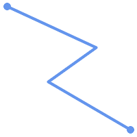(a)	(b)
(c)	(d)

A MULTILINESTRING is simple only if all of its elements are simple and the only intersection between any two elements occurs at points that are on the boundaries of both elements.

(e) and (f) are simple MULTILINESTRINGs. (g) is not simple.

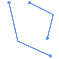(e)

(f)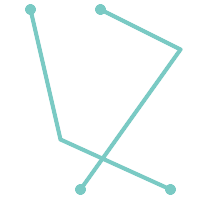

(g)

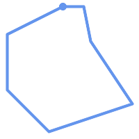
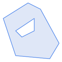
POLYGONs are formed from linear rings, so valid polygonal geometry is always simple.

To test if a geometry is simple use the ST_IsSimple function:

SELECT
   ST_IsSimple('LINESTRING(0 0, 100 100)') AS straight,
   ST_IsSimple('LINESTRING(0 0, 100 100, 100 0, 0 100)') AS crossing;

 straight | crossing
----------+----------
 t        | f

Generally, PostGIS functions do not require geometric arguments to be simple. Simplicity is primarily used as a basis for defining geometric validity. It is also a requirement for some kinds of spatial data models (for example, linear networks often disallow lines that cross). Multipoint and linear geometry can be made simple using ST_UnaryUnion.

Geometry validity primarily applies to 2-dimensional geometries (POLYGONs and MULTIPOLYGONs) . Validity is defined by rules that allow polygonal geometry to model planar areas unambiguously.

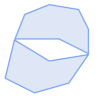
A POLYGON is valid if:

(h) and (i) are valid POLYGONs. (j-m) are invalid. (j) can be represented as a valid MULTIPOLYGON.

(h)	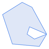(i)	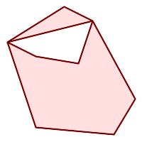(j)
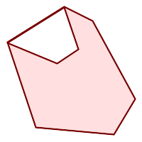(k)	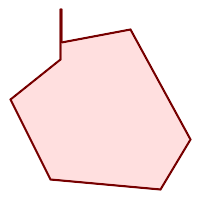(l)	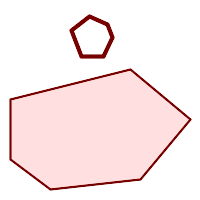(m)

A MULTIPOLYGON is valid if:

(n) is a valid MULTIPOLYGON. (o) and (p) are invalid.

(n)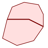

(o)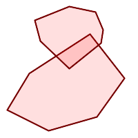

(p)

These rules mean that valid polygonal geometry is also simple.

For linear geometry the only validity rule is that LINESTRINGs must have at least two points and have non-zero length (or equivalently, have at least two distinct points.) Note that non-simple (self-intersecting) lines are valid.

SELECT
   ST_IsValid('LINESTRING(0 0, 1 1)') AS len_nonzero,
   ST_IsValid('LINESTRING(0 0, 0 0, 0 0)') AS len_zero,
   ST_IsValid('LINESTRING(10 10, 150 150, 180 50, 20 130)') AS self_int;

 len_nonzero | len_zero | self_int
-------------+----------+----------
 t           | f        | t

POINT and MULTIPOINT geometries have no validity rules.

PostGIS allows creating and storing both valid and invalid Geometry. This allows invalid geometry to be detected and flagged or fixed. There are also situations where the OGC validity rules are stricter than desired (examples of this are zero-length linestrings and polygons with inverted holes.)

Many of the functions provided by PostGIS rely on the assumption that geometry arguments are valid. For example, it does not make sense to calculate the area of a polygon that has a hole defined outside of the polygon, or to construct a polygon from a non-simple boundary line. Assuming valid geometric inputs allows functions to operate more efficiently, since they do not need to check for topological correctness. (Notable exceptions are that zero-length lines and polygons with inversions are generally handled correctly.) Also, most PostGIS functions produce valid geometry output if the inputs are valid. This allows PostGIS functions to be chained together safely.

If you encounter unexpected error messages when calling PostGIS functions (such as "GEOS Intersection() threw an error!"), you should first confirm that the function arguments are valid. If they are not, then consider using one of the techniques below to ensure the data you are processing is valid.

	If a function reports an error with valid inputs, then you may have found an error in either PostGIS or one of the libraries it uses, and you should report this to the PostGIS project. The same is true if a PostGIS function returns an invalid geometry for valid input.

To test if a geometry is valid use the ST_IsValid function:

SELECT ST_IsValid('POLYGON ((20 180, 180 180, 180 20, 20 20, 20 180))');
-----------------
 t

Information about the nature and location of an geometry invalidity are provided by the ST_IsValidDetail function:

SELECT valid, reason, ST_AsText(location) AS location
    FROM ST_IsValidDetail('POLYGON ((20 20, 120 190, 50 190, 170 50, 20 20))') AS t;

 valid |      reason       |                  location
-------+-------------------+---------------------------------------------
 f     | Self-intersection | POINT(91.51162790697674 141.56976744186045)

In some situations it is desirable to correct invalid geometry automatically. Use the ST_MakeValid function to do this. (ST_MakeValid is a case of a spatial function that does allow invalid input!)

By default, PostGIS does not check for validity when loading geometry, because validity testing can take a lot of CPU time for complex geometries. If you do not trust your data sources, you can enforce a validity check on your tables by adding a check constraint:

ALTER TABLE mytable
  ADD CONSTRAINT geometry_valid_check
        CHECK (ST_IsValid(geom));

The SPATIAL_REF_SYS table used by PostGIS is an OGC-compliant database table that defines the available spatial reference systems. It holds the numeric SRIDs and textual descriptions of the coordinate systems.

The spatial_ref_sys table definition is:

CREATE TABLE spatial_ref_sys (
  srid       INTEGER NOT NULL PRIMARY KEY,
  auth_name  VARCHAR(256),
  auth_srid  INTEGER,
  srtext     VARCHAR(2048),
  proj4text  VARCHAR(2048)
)

The columns are:

When retrieving spatial reference system definitions for use in transformations, PostGIS uses fhe following strategy:

The PostGIS spatial_ref_sys table contains over 3000 of the most common spatial reference system definitions that are handled by the PROJ projection library. But there are many coordinate systems that it does not contain. You can add SRS definitions to the table if you have the required information about the spatial reference system. Or, you can define your own custom spatial reference system if you are familiar with PROJ constructs. Keep in mind that most spatial reference systems are regional and have no meaning when used outside of the bounds they were intended for.

A resource for finding spatial reference systems not defined in the core set is http://spatialreference.org/

Some commonly used spatial reference systems are: 4326 - WGS 84 Long Lat, 4269 - NAD 83 Long Lat, 3395 - WGS 84 World Mercator, 2163 - US National Atlas Equal Area, and the 60 WGS84 UTM zones. UTM zones are one of the most ideal for measurement, but only cover 6-degree regions. (To determine which UTM zone to use for your area of interest, see the utmzone PostGIS plpgsql helper function.)

US states use State Plane spatial reference systems (meter or feet based) - usually one or 2 exists per state. Most of the meter-based ones are in the core set, but many of the feet-based ones or ESRI-created ones will need to be copied from spatialreference.org.

You can even define non-Earth-based coordinate systems, such as Mars 2000 This Mars coordinate system is non-planar (it's in degrees spheroidal), but you can use it with the geography type to obtain length and proximity measurements in meters instead of degrees.

Here is an example of loading a custom coordinate system using an unassigned SRID and the PROJ definition for a US-centric Lambert Conformal projection:

INSERT INTO spatial_ref_sys (srid, proj4text)
VALUES ( 990000,
  '+proj=lcc  +lon_0=-95 +lat_0=25 +lat_1=25 +lat_2=25 +x_0=0 +y_0=0 +datum=WGS84 +units=m +no_defs'
);

You can create a table to store geometry data using the CREATE TABLE SQL statement with a column of type geometry. The following example creates a table with a geometry column storing 2D (XY) LineStrings in the BC-Albers coordinate system (SRID 3005):

CREATE TABLE roads (
    id SERIAL PRIMARY KEY,
    name VARCHAR(64),
    geom geometry(LINESTRING,3005)
  );

The geometry type supports two optional type modifiers:

Examples of creating tables with geometry columns:

It is possible to have more than one geometry column in a table. This can be specified when the table is created, or a column can be added using the ALTER TABLE SQL statement. This example adds a column that can hold 3D LineStrings:

ALTER TABLE roads ADD COLUMN geom2 geometry(LINESTRINGZ,4326);

The OGC Simple Features Specification for SQL defines the GEOMETRY_COLUMNS metadata table to describe geometry table structure. In PostGIS geometry_columns is a view reading from database system catalog tables. This ensures that the spatial metadata information is always consistent with the currently defined tables and views. The view structure is:

\d geometry_columns

View "public.geometry_columns"
      Column       |          Type          | Modifiers
-------------------+------------------------+-----------
 f_table_catalog   | character varying(256) |
 f_table_schema    | character varying(256) |
 f_table_name      | character varying(256) |
 f_geometry_column | character varying(256) |
 coord_dimension   | integer                |
 srid              | integer                |
 type              | character varying(30)  |

The columns are:

Zwei Fälle bei denen Sie dies benötigen könnten sind SQL-Views und Masseninserts. Beim Fall von Masseninserts können Sie die Registrierung in der Tabelle "geometry_columns" korrigieren, indem Sie auf die Spalte einen CONSTRAINT setzen oder ein "ALTER TABLE" durchführen. Falls Ihre Spalte Typmod basiert ist, geschieht die Registrierung beim Erstellungsprozess auf korrekte Weise, so dass Sie hier nichts tun müssen. Auch Views, bei denen keine räumliche Funktion auf die Geometrie angewendet wird, werden auf gleiche Weise wie die Geometrie der zugrunde liegenden Tabelle registriert.

-- Lets say you have a view created like this
CREATE VIEW public.vwmytablemercator AS
        SELECT gid, ST_Transform(geom, 3395) As geom, f_name
        FROM public.mytable;

-- For it to register correctly
-- You need to cast the geometry
--
DROP VIEW public.vwmytablemercator;
CREATE VIEW  public.vwmytablemercator AS
        SELECT gid, ST_Transform(geom, 3395)::geometry(Geometry, 3395) As geom, f_name
        FROM public.mytable;

-- If you know the geometry type for sure is a 2D POLYGON then you could do
DROP VIEW public.vwmytablemercator;
CREATE VIEW  public.vwmytablemercator AS
        SELECT gid, ST_Transform(geom,3395)::geometry(Polygon, 3395) As geom, f_name
        FROM public.mytable;

--Lets say you created a derivative table by doing a bulk insert
SELECT poi.gid, poi.geom, citybounds.city_name
INTO myschema.my_special_pois
FROM poi INNER JOIN citybounds ON ST_Intersects(citybounds.geom, poi.geom);

-- Create 2D index on new table
CREATE INDEX idx_myschema_myspecialpois_geom_gist
  ON myschema.my_special_pois USING gist(geom);

-- If your points are 3D points or 3M points,
-- then you might want to create an nd index instead of a 2D index
CREATE INDEX my_special_pois_geom_gist_nd
        ON my_special_pois USING gist(geom gist_geometry_ops_nd);

-- To manually register this new table's geometry column in geometry_columns.
-- Note it will also change the underlying structure of the table to
-- to make the column typmod based.
SELECT populate_geometry_columns('myschema.my_special_pois'::regclass);

-- If you are using PostGIS 2.0 and for whatever reason, you
-- you need the constraint based definition behavior
-- (such as case of inherited tables where all children do not have the same type and srid)
-- set optional use_typmod argument to false
SELECT populate_geometry_columns('myschema.my_special_pois'::regclass, false); 

Obwohl die alte auf CONSTRAINTs basierte Methode immer noch unterstützt wird, wird eine auf Constraints basierende Geometriespalte, die direkt in einem View verwendet wird, nicht korrekt in geometry_columns registriert. Eine Typmod basierte wird korrekt registriert. Im folgenden Beispiel definieren wir eine Spalte mit Typmod und eine andere mit Constraints.

CREATE TABLE pois_ny(gid SERIAL PRIMARY KEY, poi_name text, cat text, geom geometry(POINT,4326));
SELECT AddGeometryColumn('pois_ny', 'geom_2160', 2160, 'POINT', 2, false);

In psql:

\d pois_ny;

Wir sehen, das diese Spalten unterschiedlich definiert sind -- eine mittels Typmodifizierer, eine nutzt einen Constraint

Table "public.pois_ny"
  Column   |         Type          |                       Modifiers

-----------+-----------------------+------------------------------------------------------
 gid       | integer               | not null default nextval('pois_ny_gid_seq'::regclass)
 poi_name  | text                  |
 cat       | character varying(20) |
 geom      | geometry(Point,4326)  |
 geom_2160 | geometry              |
Indexes:
    "pois_ny_pkey" PRIMARY KEY, btree (gid)
Check constraints:
    "enforce_dims_geom_2160" CHECK (st_ndims(geom_2160) = 2)
    "enforce_geotype_geom_2160" CHECK (geometrytype(geom_2160) = 'POINT'::text
        OR geom_2160 IS NULL)
    "enforce_srid_geom_2160" CHECK (st_srid(geom_2160) = 2160)

Beide registrieren sich korrekt in "geometry_columns"

SELECT f_table_name, f_geometry_column, srid, type
        FROM geometry_columns
        WHERE f_table_name = 'pois_ny';

f_table_name | f_geometry_column | srid | type
-------------+-------------------+------+-------
pois_ny      | geom              | 4326 | POINT
pois_ny      | geom_2160         | 2160 | POINT

Jedoch -- wenn wir einen View auf die folgende Weise erstellen

CREATE VIEW vw_pois_ny_parks AS
SELECT *
  FROM pois_ny
  WHERE cat='park';

SELECT f_table_name, f_geometry_column, srid, type
        FROM geometry_columns
        WHERE f_table_name = 'vw_pois_ny_parks';

Die Typmod basierte geometrische Spalte eines View registriert sich korrekt, die auf Constraint basierende nicht.

f_table_name   | f_geometry_column | srid |   type
------------------+-------------------+------+----------
 vw_pois_ny_parks | geom              | 4326 | POINT
 vw_pois_ny_parks | geom_2160         |    0 | GEOMETRY

This may change in future versions of PostGIS, but for now to force the constraint-based view column to register correctly, you need to do this:

DROP VIEW vw_pois_ny_parks;
CREATE VIEW vw_pois_ny_parks AS
SELECT gid, poi_name, cat,
  geom,
  geom_2160::geometry(POINT,2160) As geom_2160
  FROM pois_ny
  WHERE cat = 'park';
SELECT f_table_name, f_geometry_column, srid, type
        FROM geometry_columns
        WHERE f_table_name = 'vw_pois_ny_parks';

f_table_name   | f_geometry_column | srid | type
------------------+-------------------+------+-------
 vw_pois_ny_parks | geom              | 4326 | POINT
 vw_pois_ny_parks | geom_2160         | 2160 | POINT

If spatial data can be converted to a text representation (as either WKT or WKB), then using SQL might be the easiest way to get data into PostGIS. Data can be bulk-loaded into PostGIS/PostgreSQL by loading a text file of SQL INSERT statements using the psql SQL utility.

A SQL load file (roads.sql for example) might look like this:

BEGIN;
INSERT INTO roads (road_id, roads_geom, road_name)
  VALUES (1,'LINESTRING(191232 243118,191108 243242)','Jeff Rd');
INSERT INTO roads (road_id, roads_geom, road_name)
  VALUES (2,'LINESTRING(189141 244158,189265 244817)','Geordie Rd');
INSERT INTO roads (road_id, roads_geom, road_name)
  VALUES (3,'LINESTRING(192783 228138,192612 229814)','Paul St');
INSERT INTO roads (road_id, roads_geom, road_name)
  VALUES (4,'LINESTRING(189412 252431,189631 259122)','Graeme Ave');
INSERT INTO roads (road_id, roads_geom, road_name)
  VALUES (5,'LINESTRING(190131 224148,190871 228134)','Phil Tce');
INSERT INTO roads (road_id, roads_geom, road_name)
  VALUES (6,'LINESTRING(198231 263418,198213 268322)','Dave Cres');
COMMIT;

The SQL file can be loaded into PostgreSQL using psql:

psql -d [database] -f roads.sql

The shp2pgsql data loader converts Shapefiles into SQL suitable for insertion into a PostGIS/PostgreSQL database either in geometry or geography format. The loader has several operating modes selected by command line flags.

There is also a shp2pgsql-gui graphical interface with most of the options as the command-line loader. This may be easier to use for one-off non-scripted loading or if you are new to PostGIS. It can also be configured as a plugin to PgAdminIII.

An example session using the loader to create an input file and loading it might look like this:

# shp2pgsql -c -D -s 4269 -i -I shaperoads.shp myschema.roadstable > roads.sql
# psql -d roadsdb -f roads.sql

A conversion and load can be done in one step using UNIX pipes:

# shp2pgsql shaperoads.shp myschema.roadstable | psql -d roadsdb

The most straightforward way of extracting spatial data out of the database is to use a SQL SELECT query to define the data set to be extracted and dump the resulting columns into a parsable text file:

db=# SELECT road_id, ST_AsText(road_geom) AS geom, road_name FROM roads;

road_id | geom                                    | road_name
--------+-----------------------------------------+-----------
          1 | LINESTRING(191232 243118,191108 243242) | Jeff Rd
          2 | LINESTRING(189141 244158,189265 244817) | Geordie Rd
          3 | LINESTRING(192783 228138,192612 229814) | Paul St
          4 | LINESTRING(189412 252431,189631 259122) | Graeme Ave
          5 | LINESTRING(190131 224148,190871 228134) | Phil Tce
          6 | LINESTRING(198231 263418,198213 268322) | Dave Cres
          7 | LINESTRING(218421 284121,224123 241231) | Chris Way
(6 rows)

There will be times when some kind of restriction is necessary to cut down the number of records returned. In the case of attribute-based restrictions, use the same SQL syntax as used with a non-spatial table. In the case of spatial restrictions, the following functions are useful:

Außerdem können Sie diese Operatoren in Anfragen verwenden. Beachten Sie bitte, wenn Sie eine Geometrie oder eine Box auf der SQL-Befehlszeile eingeben, dass Sie die Zeichensatzdarstellung explizit in eine Geometrie umwandeln müssen. 312 ist ein fiktives Koordinatenreferenzsystem das zu unseren Daten passt. Also, zum Beispiel:

SELECT road_id, road_name
  FROM roads
  WHERE roads_geom='SRID=312;LINESTRING(191232 243118,191108 243242)'::geometry;

Die obere Abfrage würde einen einzelnen Datensatz aus der Tabelle "ROADS_GEOM" zurückgeben, in dem die Geometrie gleich dem angegebenen Wert ist.

Überprüfung ob einige der Strassen in die Polygonfläche hineinreichen:

SELECT road_id, road_name
FROM roads
WHERE ST_Intersects(roads_geom, 'SRID=312;POLYGON((...))');

Die häufigsten räumlichen Abfragen werden vermutlich in einem bestimmten Ausschnitt ausgeführt. Insbesondere von Client-Software, wie Datenbrowsern und Kartendiensten, die auf diese Weise die Daten für die Darstellung eines "Kartenausschnitts" erfassen.

Der Operator "&&" kann entweder mit einer BOX3D oder mit einer Geometrie verwendet werden. Allerdings wird auch bei einer Geometrie nur das Umgebungsrechteck für den Vergleich herangezogen.

Die Abfrage zur Verwendung des "BOX3D" Objekts für einen solchen Ausschnitt sieht folgendermaßen aus:

SELECT ST_AsText(roads_geom) AS geom
FROM roads
WHERE
  roads_geom && ST_MakeEnvelope(191232, 243117,191232, 243119,312);

Achten Sie auf die Verwendung von SRID=312, welche die Projektion Einhüllenden/Enveloppe bestimmt.

The pgsql2shp table dumper connects to the database and converts a table (possibly defined by a query) into a shape file. The basic syntax is:

pgsql2shp [<options>] <database> [<schema>.]<table>

pgsql2shp [<options>] <database> <query>

Optionen auf der Befehlszeile:

GiST stands for "Generalized Search Tree" and is a generic form of indexing for multi-dimensional data. PostGIS uses an R-Tree index implemented on top of GiST to index spatial data. GiST is the most commonly-used and versatile spatial index method, and offers very good query performance. Other implementations of GiST are used to speed up searches on all kinds of irregular data structures (integer arrays, spectral data, etc) which are not amenable to normal B-Tree indexing. For more information see the PostgreSQL manual.

Once a spatial data table exceeds a few thousand rows, you will want to build an index to speed up spatial searches of the data (unless all your searches are based on attributes, in which case you'll want to build a normal index on the attribute fields).

Die Syntax, mit der ein GIST-Index auf eine Geometriespalte gelegt wird, lautet:

CREATE INDEX [indexname] ON [tablename] USING GIST ( [geometryfield] ); 

Die obere Syntax erzeugt immer einen 2D-Index. Um einen n-dimensionalen Index für den geometrischen Datentyp zu erhalten, können Sie die folgende Syntax verwenden:

CREATE INDEX [indexname] ON [tablename] USING GIST ([geometryfield] gist_geometry_ops_nd);

Die Erstellung eines räumlichen Indizes ist eine rechenintensive Aufgabe. Während der Erstellung wird auch der Schreibzugriff auf die Tabelle blockiert. Bei produktiven Systemen empfiehlt sich daher die langsamere Option CONCURRENTLY:

CREATE INDEX CONCURRENTLY [indexname] ON [tablename] USING GIST ( [geometryfield] ); 

Nachdem ein Index aufgebaut wurde sollte PostgreSQL gezwungen werden die Tabellenstatistik zu sammeln, da diese zur Optmierung der Auswertungspläne verwendet wird:

VACUUM ANALYZE [table_name] [(column_name)];

BRIN stands for "Block Range Index". It is a general-purpose index method introduced in PostgreSQL 9.5. BRIN is a lossy index method, meaning that a secondary check is required to confirm that a record matches a given search condition (which is the case for all provided spatial indexes). It provides much faster index creation and much smaller index size, with reasonable read performance. Its primary purpose is to support indexing very large tables on columns which have a correlation with their physical location within the table. In addition to spatial indexing, BRIN can speed up searches on various kinds of attribute data structures (integer, arrays etc). For more information see the PostgreSQL manual.

Once a spatial table exceeds a few thousand rows, you will want to build an index to speed up spatial searches of the data. GiST indexes are very performant as long as their size doesn't exceed the amount of RAM available for the database, and as long as you can afford the index storage size, and the cost of index update on write. Otherwise, for very large tables BRIN index can be considered as an alternative.

A BRIN index stores the bounding box enclosing all the geometries contained in the rows in a contiguous set of table blocks, called a block range. When executing a query using the index the block ranges are scanned to find the ones that intersect the query extent. This is efficient only if the data is physically ordered so that the bounding boxes for block ranges have minimal overlap (and ideally are mutually exclusive). The resulting index is very small in size, but is typically less performant for read than a GiST index over the same data.

Building a BRIN index is much less CPU-intensive than building a GiST index. It's common to find that a BRIN index is ten times faster to build than a GiST index over the same data. And because a BRIN index stores only one bounding box for each range of table blocks, it's common to use up to a thousand times less disk space than a GiST index.

You can choose the number of blocks to summarize in a range. If you decrease this number, the index will be bigger but will probably provide better performance.

For BRIN to be effective, the table data should be stored in a physical order which minimizes the amount of block extent overlap. It may be that the data is already sorted appropriately (for instance, if it is loaded from another dataset that is already sorted in spatial order). Otherwise, this can be accomplished by sorting the data by a one-dimensional spatial key. One way to do this is to create a new table sorted by the geometry values (which in recent PostGIS versions uses an efficient Hilbert curve ordering):

CREATE TABLE table_sorted AS
   SELECT * FROM table  ORDER BY geom;

Alternatively, data can be sorted in-place by using a GeoHash as a (temporary) index, and clustering on that index:

CREATE INDEX idx_temp_geohash ON table
    USING btree (ST_GeoHash( ST_Transform( geom, 4326 ), 20));
CLUSTER table USING idx_temp_geohash;

The syntax for building a BRIN index on a geometry column is:

CREATE INDEX [indexname] ON [tablename] USING BRIN ( [geome_col] ); 

The above syntax builds a 2D index. To build a 3D-dimensional index, use this syntax:

CREATE INDEX [indexname] ON [tablename]
    USING BRIN ([geome_col] brin_geometry_inclusion_ops_3d);

You can also get a 4D-dimensional index using the 4D operator class:

CREATE INDEX [indexname] ON [tablename]
    USING BRIN ([geome_col] brin_geometry_inclusion_ops_4d);

The above commands use the default number of blocks in a range, which is 128. To specify the number of blocks to summarise in a range, use this syntax

CREATE INDEX [indexname] ON [tablename]
    USING BRIN ( [geome_col] ) WITH (pages_per_range = [number]); 

Keep in mind that a BRIN index only stores one index entry for a large number of rows. If your table stores geometries with a mixed number of dimensions, it's likely that the resulting index will have poor performance. You can avoid this performance penalty by choosing the operator class with the least number of dimensions of the stored geometries

The geography datatype is supported for BRIN indexing. The syntax for building a BRIN index on a geography column is:

CREATE INDEX [indexname] ON [tablename] USING BRIN ( [geog_col] ); 

The above syntax builds a 2D-index for geospatial objects on the spheroid.

Currently, only "inclusion support" is provided, meaning that just the &&, ~ and @ operators can be used for the 2D cases (for both geometry and geography), and just the &&& operator for 3D geometries. There is currently no support for kNN searches.

An important difference between BRIN and other index types is that the database does not maintain the index dynamically. Changes to spatial data in the table are simply appended to the end of the index. This will cause index search performance to degrade over time. The index can be updated by performing a VACUUM, or by using a special function brin_summarize_new_values(regclass). For this reason BRIN may be most appropriate for use with data that is read-only, or only rarely changing. For more information refer to the manual.

To summarize using BRIN for spatial data:

SP-GiST stands for "Space-Partitioned Generalized Search Tree" and is a generic form of indexing for multi-dimensional data types that supports partitioned search trees, such as quad-trees, k-d trees, and radix trees (tries). The common feature of these data structures is that they repeatedly divide the search space into partitions that need not be of equal size. In addition to spatial indexing, SP-GiST is used to speed up searches on many kinds of data, such as phone routing, ip routing, substring search, etc. For more information see the PostgreSQL manual.

As it is the case for GiST indexes, SP-GiST indexes are lossy, in the sense that they store the bounding box enclosing spatial objects. SP-GiST indexes can be considered as an alternative to GiST indexes.

Sobald eine Geodatentabelle einige tausend Zeilen überschreitet, kann es sinnvoll sein einen SP-GIST Index zu erzeugen, um die räumlichen Abfragen auf die Daten zu beschleunigen. Die Syntax zur Erstellung eines SP-GIST Index auf eine "Geometriespalte" lautet:

CREATE INDEX [indexname] ON [tablename] USING SPGIST ( [geometryfield] ); 

Die obere Syntax erzeugt einen 2D-Index. Ein 3-dimensionaler Index für den geometrischen Datentyp können Sie mit der 3D Operatorklasse erstellen:

CREATE INDEX [indexname] ON [tablename] USING SPGIST ([geometryfield] spgist_geometry_ops_3d);

Die Erstellung eines räumlichen Indizes ist eine rechenintensive Aufgabe. Während der Erstellung wird auch der Schreibzugriff auf die Tabelle blockiert. Bei produktiven Systemen empfiehlt sich daher die langsamere Option CONCURRENTLY:

CREATE INDEX CONCURRENTLY [indexname] ON [tablename] USING SPGIST ( [geometryfield] ); 

Nachdem ein Index aufgebaut wurde sollte PostgreSQL gezwungen werden die Tabellenstatistik zu sammeln, da diese zur Optmierung der Auswertungspläne verwendet wird:

VACUUM ANALYZE [table_name] [(column_name)];

Ein SP-GiST Index kann Abfragen mit folgenden Operatoren beschleunigen:

kNN Suche wird zurzeit nicht unterstützt.

Ordinarily, indexes invisibly speed up data access: once an index is built, the PostgreSQL query planner automatically decides when to use it to improve query performance. But there are some situations where the planner does not choose to use existing indexes, so queries end up using slow sequential scans instead of a spatial index.

If you find your spatial indexes are not being used, there are a few things you can do:

For more information see the Postgres manual section on Query Planning.