5. Almacenando datos espaciales¶

Soportado por una amplia variedad de bibliotecas y aplicaciones, PostGIS proporciona muchas opciones para cargar datos.

Primero cargaremos nuestros datos de trabajo desde un archivo de respaldo de base de datos, luego revisaremos algunas formas estándar de cargar diferentes formatos de datos GIS usando herramientas comunes.

5.1. Cargando el archivo de respaldo¶

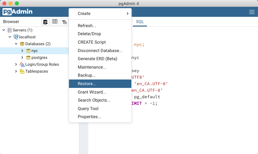
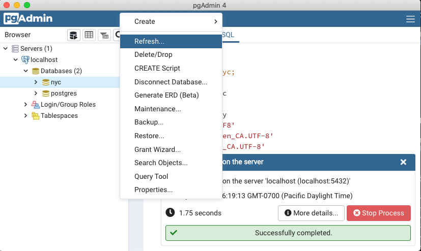
En el navegador de PgAdmin, haz clic derecho en el ícono de la base de datos nyc, y luego selecciona la opción Restore….
Browse to the location of your workshop data data directory (available in the workshop data bundle), and select the nyc_data.backup file.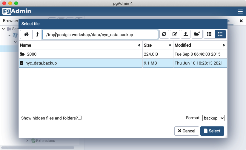
Haz clic en la pestaña Restore options, desplázate hacia abajo hasta la sección Do not save y cambia Owner a Yes.
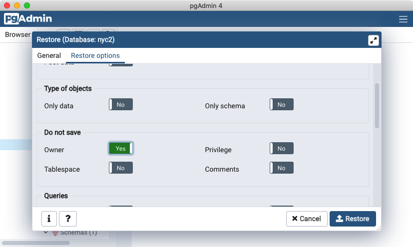
Haz clic en el botón Restore. La restauración de la base de datos debería completarse sin errores.
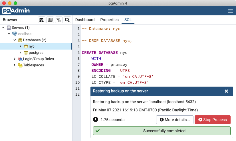
Después de que la carga se complete, haz clic derecho en la base de datos nyc, y selecciona la opción Refresh para actualizar la información del cliente acerca de qué tablas existen en la base de datos.

Nota

Si deseas practicar cargando datos desde los formatos espaciales nativos, en lugar de usar los archivos de respaldo de PostgreSQL recién cubiertos, las siguientes secciones te guiarán a través de la carga usando varias herramientas de línea de comandos y QGIS DbManager. Nota que puedes omitir estas secciones si ya has cargado los datos con pgAdmin.

5.2. Cargando con ogr2ogr¶

ogr2ogr es una utilidad de línea de comandos para convertir datos entre formatos de datos GIS, incluyendo formatos de archivo comunes y bases de datos espaciales comunes.

Windows:

Las compilaciones de ogr2ogr se pueden descargar desde GIS Internals.
ogr2ogr está incluido como parte de QGIS Install y accesible mediante OSGeo4W Shell -
Las compilaciones de ogr2ogr se pueden descargar desde MS4W.

MacOS:

Si instalaste Postgres.app, entonces encontrarás ogr2ogr en el directorio /Applications/Postgres.app/Contents/Versions/*/bin.
Finalmente, si instalaste HomeBrew puedes instalar el paquete gdal para tener acceso a ogr2ogr

Linux:

Si instalaste QGIS desde paquetes, ogr2ogr debería estar instalado y en tu PATH ya como parte de los paquetes gdal o libgdal.

El directorio de datos del taller de postgis incluye un subdirectorio 2000/, que contiene archivos shape del censo 2000, que fueron reemplazados por datos del censo 2010. Podemos practicar la carga de datos usando esos archivos, para evitar crear colisiones de nombres con los datos que ya cargamos usando el archivo de respaldo. Asegúrate de estar en el subdirectorio 2000/ con la shell al hacer estas instrucciones:

export PGPASSWORD=mydatabasepassword

En lugar de pasar la contraseña en la cadena de conexión, la colocamos en el entorno, para que no sea visible en la lista de procesos mientras se ejecuta el comando.

Ten en cuenta que en Windows, deberás usar set en lugar de export.

ogr2ogr \
  -nln nyc_census_blocks_2000 \
  -nlt PROMOTE_TO_MULTI \
  -lco GEOMETRY_NAME=geom \
  -lco FID=gid \
  -lco PRECISION=NO \
  Pg:"dbname=nyc host=localhost user=pramsey port=5432" \
  nyc_census_blocks_2000.shp

Para mayor claridad visual, estas líneas se muestran con \, pero deben escribirse en una sola línea en tu shell.

El ogr2ogr tiene una cantidad enorme de opciones, y aquí solo estamos usando unas pocas. Aquí tienes una explicación línea por línea del comandos.

ogr2ogr \

¡El nombre del ejecutable! Es posible que necesites asegurarte de que la ubicación del ejecutable esté en tu PATH o usar la ruta completa al ejecutable, dependiendo de tu configuración.

-nln nyc_census_blocks_2000 \

La opción nln significa «new layer name», y establece el nombre de la tabla que se creará en la base de datos de destino.

-nlt PROMOTE_TO_MULTI \

La opción nlt significa «new layer type». Para entrada de archivos shape en particular, el nuevo tipo de capa suele ser una «geometría de múltiples partes», por lo que el sistema necesita que se le indique de antemano que use «MultiPolygon» en lugar de «Polygon» para el tipo de geometría.

-lco GEOMETRY_NAME=geom \
-lco FID=gid \
-lco PRECISION=NO \

La opción lco significa «layer create option». Los distintos controladores tienen diferentes opciones de creación, y aquí estamos usando tres opciones para el PostgreSQL driver.

GEOMETRY_NAME establece el nombre de la columna para la columna de geometría. Preferimos «geom» sobre el valor por defecto, para que nuestras tablas coincidan con los nombres de columna estándar en el taller.
FID establece el nombre de la columna de clave primaria. Nuevamente, preferimos «gid», que es el estándar usado en el taller.
PRECISION controla cómo se representan los campos numéricos en la base de datos. El valor por defecto al cargar un archivo shape es usar el tipo «numeric» de la base de datos, que es más preciso pero a veces más difícil de manejar que los tipos numéricos simples como «integer» y «double precision». Usamos «NO» para desactivar el tipo «numeric».

Pg:"dbname=nyc host=localhost user=pramsey port=5432" \

El orden de los argumentos en ogr2ogr es, aproximadamente: ejecutable, luego opciones, luego la ubicación de destino, y luego la ubicación de origen. Así que este es el destino, la cadena de conexión para nuestra base de datos PostgreSQL. La parte «Pg:» es el nombre del controlador, y luego la connection string está contenida entre comillas (porque puede tener espacios incrustados).

nyc_census_blocks_2000.shp

El conjunto de datos de origen en este caso es el archivo shape que estamos leyendo. Es posible leer múltiples capas en una sola invocación colocando la cadena de conexión aquí, y luego siguiéndola con una lista de nombres de capas, pero en este caso solo tenemos un archivo shape para cargar.

5.3. ¿Shapefiles? ¿Qué es eso?¶

Podrías estar preguntándote — «¿Qué es este archivo shapefile?» Un «shapefile» comúnmente se refiere a una colección de archivos con extensiones .shp, .shx, .dbf y otras, con un nombre de prefijo común (ejemplo, nyc_census_blocks). El archivo shapefile en realidad se refiere específicamente a los archivos con extensión .shp. Sin embargo, el archivo .shp por sí solo está incompleto para distribución sin los archivos de soporte requeridos.

Archivos obligatorios:

.shp—formato shape; la geometría de la entidad en sí
.shx—formato de índice shape; un índice posicional de la geometría de la entidad
.dbf—formato de atributos; atributos en columnas para cada shape, en dBase III

Los archivos opcionales incluyen:

.prj—formato de proyección; el sistema de coordenadas e información de proyección, un archivo de texto plano que describe la proyección usando el formato well-known text

La utilidad shp2pgsql hace que los datos shape sean utilizables en PostGIS al convertirlos de datos binarios a una serie de comandos SQL que luego se ejecutan en la base de datos para cargar los datos.

5.4. Cargando con shp2pgsql¶

shp2pgsql convierte archivos Shape en SQL. Es una utilidad de conversión que forma parte del núcleo de PostGIS y se distribuye con los paquetes de PostGIS. Si instalaste PostgreSQL localmente en tu computadora, es posible que encuentres que shp2pgsql fue instalado junto con él, y que está disponible en el directorio de ejecutables de tu instalación.

A diferencia de ogr2ogr, shp2pgsql no se conecta directamente a la base de datos de destino, simplemente emite el SQL equivalente al archivo shape de entrada. Depende del usuario pasar el SQL a la base de datos, ya sea con un «pipe» o guardando el SQL en un archivo y luego cargándolo.

Aquí tienes un ejemplo de invocación, cargando los mismos datos que antes:

export PGPASSWORD=mydatabasepassword

shp2pgsql \
  -D \
  -I \
  -s 26918 \
  nyc_census_blocks_2000.shp \
  nyc_census_blocks_2000 \
  | psql dbname=nyc user=postgres host=localhost

Aquí tienes una explicación línea por línea del comando.

shp2pgsql \

¡El programa ejecutable! Lee el archivo de datos de origen y emite SQL que puede dirigirse a un archivo o canalizarse a psql para cargar directamente en la base de datos.

-D \

La bandera D le dice al programa que genere «dump format» que es mucho más rápido de cargar que el «insert format» de manera predeterminada.

-I \

La bandera I le dice al programa que cree un índice espacial en la tabla después de que se complete la carga.

-s 26918 \

La bandera s le dice al programa cuál es el «identificador de referencia espacial (SRID)» de los datos. Los datos de origen de este taller están todos en «UTM 18», para lo cual el SRID es 26918 (ver más abajo).

nyc_census_blocks_2000.shp \

El archivo shape de origen a leer.

nyc_census_blocks_2000 \

El nombre de la tabla a usar al crear la tabla de destino.

| psql dbname=nyc user=postgres host=localhost

El programa utilitario está generando un flujo de SQL. El operador «|» toma ese flujo y lo usa como entrada para el programa de terminal de base de datos psql. Los argumentos para psql son simplemente la cadena de conexión para la base de datos de destino.

5.5. ¿SRID 26918? ¿Qué significa eso?¶

La mayor parte del proceso de importación es autoexplicativa, pero incluso los profesionales GIS con experiencia pueden tropezar con un SRID.

Un «SRID» significa «Spatial Reference IDentifier» (Identificador de Referencia Espacial). Define todos los parámetros del sistema de coordenadas geográficas y la proyección de nuestros datos. Un SRID es conveniente porque empaqueta toda la información sobre una proyección cartográfica (que puede ser bastante compleja) en un solo número.

Puedes ver la definición de nuestra proyección de mapa del taller consultándola en una base de datos en línea,

https://epsg.io/26918

o directamente dentro de PostGIS con una consulta a la tabla spatial_ref_sys.

SELECT srtext FROM spatial_ref_sys WHERE srid = 26918;

Nota

La tabla spatial_ref_sys de PostGIS es una tabla estándar OGC que define todos los sistemas de referencia espacial conocidos por la base de datos. Los datos que se distribuyen con PostGIS listan más de 3000 sistemas de referencia espacial conocidos y los detalles necesarios para transformarlos/reproyectarlos entre sí.

En ambos casos, ves una representación textual del sistema de referencia espacial 26918 (impreso aquí con formato para mayor claridad):

PROJCS["NAD83 / UTM zone 18N",
  GEOGCS["NAD83",
    DATUM["North_American_Datum_1983",
      SPHEROID["GRS 1980",6378137,298.257222101,AUTHORITY["EPSG","7019"]],
      AUTHORITY["EPSG","6269"]],
    PRIMEM["Greenwich",0,AUTHORITY["EPSG","8901"]],
    UNIT["degree",0.01745329251994328,AUTHORITY["EPSG","9122"]],
    AUTHORITY["EPSG","4269"]],
  UNIT["metre",1,AUTHORITY["EPSG","9001"]],
  PROJECTION["Transverse_Mercator"],
  PARAMETER["latitude_of_origin",0],
  PARAMETER["central_meridian",-75],
  PARAMETER["scale_factor",0.9996],
  PARAMETER["false_easting",500000],
  PARAMETER["false_northing",0],
  AUTHORITY["EPSG","26918"],
  AXIS["Easting",EAST],
  AXIS["Northing",NORTH]]

Si abres el archivo nyc_neighborhoods.prj del directorio de datos, verás la misma definición de proyección.

Los datos que recibes de agencias locales—como la Ciudad de Nueva York—usualmente estarán en una proyección local indicada como «state plane» o «UTM». Nuestra proyección es «Universal Transverse Mercator (UTM) Zona 18 Norte» o EPSG:26918.

5.6. Cosas para probar: Ver datos usando QGIS¶

QGIS, es un visor/editor GIS de escritorio para observar rápidamente los datos. Puedes ver numerosos formatos de datos incluyendo shapefiles planos y una base de datos PostGIS. Su interfaz gráfica permite una exploración sencilla de tus datos, así como pruebas simples y un estilizado rápido.

Intenta usar este software para conectarte a tu base de datos PostGIS. La aplicación se puede descargar desde https://qgis.org

Primero querrás crear una conexión a una base de datos PostGIS usando el menú Layer->Add Layer->PostGIS Layers->New y luego completando las indicaciones. Una vez que tengas una conexión, puedes añadir capas haciendo clic en «connect» y seleccionando una tabla para mostrar.

5.7. Cargando datos usando QGIS DbManager¶

QGIS viene con una herramienta llamada DbManager que te permite conectarte a varios tipos de bases de datos, incluyendo una habilitada con PostGIS. Después de que tengas configurada una conexión a una base de datos PostGIS, ve a Database->DbManager y expande tu base de datos como se muestra abajo:

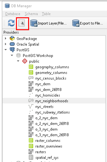
Desde ahí puedes usar la opción de menú Import Layer/File para cargar numerosos formatos espaciales diferentes. Además de poder cargar datos desde muchos formatos espaciales y exportar datos a muchos formatos, también puedes añadir consultas ad-hoc al lienzo o definir vistas en tu base de datos, usando el ícono de llave inglesa resaltado.