The Open Geospatial Consortium (OGC) developed the Simple Features Access standard (SFA) to provide a model for geospatial data. It defines the fundamental spatial type of Geometry, along with operations which manipulate and transform geometry values to perform spatial analysis tasks. PostGIS implements the OGC Geometry model as the PostgreSQL data types geometry and geography.
Geometry is an abstract type. Geometry values belong to one of its concrete subtypes which represent various kinds and dimensions of geometric shapes. These include the atomic types Point, LineString, LinearRing and Polygon, and the collection types MultiPoint, MultiLineString, MultiPolygon and GeometryCollection. The Simple Features Access - Part 1: Common architecture v1.2.1 adds subtypes for the structures PolyhedralSurface, Triangle and TIN.
Geometry models shapes in the 2-dimensional Cartesian plane. The PolyhedralSurface, Triangle, and TIN types can also represent shapes in 3-dimensional space. The size and location of shapes are specified by their coordinates. Each coordinate has a X and Y ordinate value determining its location in the plane. Shapes are constructed from points or line segments, with points specified by a single coordinate, and line segments by two coordinates.
Coordinates may contain optional Z and M ordinate values. The Z ordinate is often used to represent elevation. The M ordinate contains a measure value, which may represent time or distance. If Z or M values are present in a geometry value, they must be defined for each point in the geometry. If a geometry has Z or M ordinates the coordinate dimension is 3D; if it has both Z and M the coordinate dimension is 4D.
Geometry values are associated with a spatial reference system indicating the coordinate system in which it is embedded. The spatial reference system is identified by the geometry SRID number. The units of the X and Y axes are determined by the spatial reference system. In planar reference systems the X and Y coordinates typically represent easting and northing, while in geodetic systems they represent longitude and latitude. SRID 0 represents an infinite Cartesian plane with no units assigned to its axes. See Section 4.5, “Spatial Reference Systems”.
The geometry dimension is a property of geometry types. Point types have dimension 0, linear types have dimension 1, and polygonal types have dimension 2. Collections have the dimension of the maximum element dimension.
A geometry value may be empty. Empty values contain no vertices (for atomic geometry types) or no elements (for collections).
An important property of geometry values is their spatial extent or bounding box, which the OGC model calls envelope. This is the 2 or 3-dimensional box which encloses the coordinates of a geometry. It is an efficient way to represent a geometry's extent in coordinate space and to check whether two geometries interact.
The geometry model allows evaluating topological spatial relationships as described in Section 5.1.1, “Dimensionally Extended 9-Intersection Model”. To support this the concepts of interior, boundary and exterior are defined for each geometry type. Geometries are topologically closed, so they always contain their boundary. The boundary is a geometry of dimension one less than that of the geometry itself.
The OGC geometry model defines validity rules for each geometry type. These rules ensure that geometry values represents realistic situations (e.g. it is possible to specify a polygon with a hole lying outside the shell, but this makes no sense geometrically and is thus invalid). PostGIS also allows storing and manipulating invalid geometry values. This allows detecting and fixing them if needed. See Section 4.6, “Geometry Validation”
A Point is a 0-dimensional geometry that represents a single location in coordinate space.
POINT (1 2)
POINT Z (1 2 3)
POINT ZM (1 2 3 4)
A LineString is a 1-dimensional line formed by a contiguous sequence of line segments. Each line segment is defined by two points, with the end point of one segment forming the start point of the next segment. An OGC-valid LineString has either zero or two or more points, but PostGIS also allows single-point LineStrings. LineStrings may cross themselves (self-intersect). A LineString is closed if the start and end points are the same. A LineString is simple if it does not self-intersect.
LINESTRING (1 2, 3 4, 5 6)
A LinearRing is a LineString which is both closed and simple. The first and last points must be equal, and the line must not self-intersect.
LINEARRING (0 0 0, 4 0 0, 4 4 0, 0 4 0, 0 0 0)
A Polygon is a 2-dimensional planar region, delimited by an exterior boundary (the shell) and zero or more interior boundaries (holes). Each boundary is a LinearRing.
POLYGON ((0 0 0,4 0 0,4 4 0,0 4 0,0 0 0),(1 1 0,2 1 0,2 2 0,1 2 0,1 1 0))
A MultiLineString is a collection of LineStrings. A MultiLineString is closed if each of its elements is closed.
MULTILINESTRING ( (0 0,1 1,1 2), (2 3,3 2,5 4) )
A MultiPolygon is a collection of non-overlapping, non-adjacent Polygons. Polygons in the collection may touch only at a finite number of points.
MULTIPOLYGON (((1 5, 5 5, 5 1, 1 1, 1 5)), ((6 5, 9 1, 6 1, 6 5)))
A GeometryCollection is a heterogeneous (mixed) collection of geometries.
GEOMETRYCOLLECTION ( POINT(2 3), LINESTRING(2 3, 3 4))
A PolyhedralSurface is a contiguous collection of patches or facets which share some edges. Each patch is a planar Polygon. If the Polygon coordinates have Z ordinates then the surface is 3-dimensional.
POLYHEDRALSURFACE Z (
  ((0 0 0, 0 0 1, 0 1 1, 0 1 0, 0 0 0)),
  ((0 0 0, 0 1 0, 1 1 0, 1 0 0, 0 0 0)),
  ((0 0 0, 1 0 0, 1 0 1, 0 0 1, 0 0 0)),
  ((1 1 0, 1 1 1, 1 0 1, 1 0 0, 1 1 0)),
  ((0 1 0, 0 1 1, 1 1 1, 1 1 0, 0 1 0)),
  ((0 0 1, 1 0 1, 1 1 1, 0 1 1, 0 0 1)) )
A Triangle is a polygon defined by three distinct non-collinear vertices. Because a Triangle is a polygon it is specified by four coordinates, with the first and fourth being equal.
TRIANGLE ((0 0, 0 9, 9 0, 0 0))
A TIN is a collection of non-overlapping Triangles representing a Triangulated Irregular Network.
TIN Z ( ((0 0 0, 0 0 1, 0 1 0, 0 0 0)), ((0 0 0, 0 1 0, 1 1 0, 0 0 0)) )
The ISO/IEC 13249-3 SQL Multimedia - Spatial standard (SQL/MM) extends the OGC SFA to define Geometry subtypes containing curves with circular arcs. The SQL/MM types support 3DM, 3DZ and 4D coordinates.
![[Note]](images/note.png) | |
All floating point comparisons within the SQL-MM implementation are performed to a specified tolerance, currently 1E-8. |
CircularString is the basic curve type, similar to a LineString in the linear world. A single arc segment is specified by three points: the start and end points (first and third) and some other point on the arc. To specify a closed circle the start and end points are the same and the middle point is the opposite point on the circle diameter (which is the center of the arc). In a sequence of arcs the end point of the previous arc is the start point of the next arc, just like the segments of a LineString. This means that a CircularString must have an odd number of points greater than 1.
CIRCULARSTRING(0 0, 1 1, 1 0)

CIRCULARSTRING(0 0, 4 0, 4 4, 0 4, 0 0)
A CompoundCurve is a single continuous curve that may contain both circular arc segments and linear segments. That means that in addition to having well-formed components, the end point of every component (except the last) must be coincident with the start point of the following component.
COMPOUNDCURVE( CIRCULARSTRING(0 0, 1 1, 1 0),(1 0, 0 1))
A CurvePolygon is like a polygon, with an outer ring and zero or more inner rings. The difference is that a ring can be a CircularString or CompoundCurve as well as a LineString.
As of PostGIS 1.4 PostGIS supports compound curves in a curve polygon.
CURVEPOLYGON(
  CIRCULARSTRING(0 0, 4 0, 4 4, 0 4, 0 0),
  (1 1, 3 3, 3 1, 1 1) )
Example: A CurvePolygon with the shell defined by a CompoundCurve containing a CircularString and a LineString, and a hole defined by a CircularString
CURVEPOLYGON(
  COMPOUNDCURVE( CIRCULARSTRING(0 0,2 0, 2 1, 2 3, 4 3),
                 (4 3, 4 5, 1 4, 0 0)),
CIRCULARSTRING(1.7 1, 1.4 0.4, 1.6 0.4, 1.6 0.5, 1.7 1) )A MultiCurve is a collection of curves which can include LineStrings, CircularStrings or CompoundCurves.
MULTICURVE( (0 0, 5 5), CIRCULARSTRING(4 0, 4 4, 8 4))
The OGC SFA specification defines two formats for representing geometry values for external use: Well-Known Text (WKT) and Well-Known Binary (WKB). Both WKT and WKB include information about the type of the object and the coordinates which define it.
Well-Known Text (WKT) provides a standard textual representation of spatial data. Examples of WKT representations of spatial objects are:
POINT(0 0)
POINT Z (0 0 0)
POINT ZM (0 0 0 0)
POINT EMPTY
LINESTRING(0 0,1 1,1 2)
LINESTRING EMPTY
POLYGON((0 0,4 0,4 4,0 4,0 0),(1 1, 2 1, 2 2, 1 2,1 1))
MULTIPOINT((0 0),(1 2))
MULTIPOINT Z ((0 0 0),(1 2 3))
MULTIPOINT EMPTY
MULTILINESTRING((0 0,1 1,1 2),(2 3,3 2,5 4))
MULTIPOLYGON(((0 0,4 0,4 4,0 4,0 0),(1 1,2 1,2 2,1 2,1 1)), ((-1 -1,-1 -2,-2 -2,-2 -1,-1 -1)))
GEOMETRYCOLLECTION(POINT(2 3),LINESTRING(2 3,3 4))
GEOMETRYCOLLECTION EMPTY
Input and output of WKT is provided by the functions ST_AsText and ST_GeomFromText:
text WKT = ST_AsText(geometry);
geometry = ST_GeomFromText(text WKT, SRID);
For example, a statement to create and insert a spatial object from WKT and a SRID is:
INSERT INTO geotable ( geom, name )
  VALUES ( ST_GeomFromText('POINT(-126.4 45.32)', 312), 'A Place');
Well-Known Binary (WKB) provides a portable, full-precision representation of spatial data as binary data (arrays of bytes). Examples of the WKB representations of spatial objects are:
WKT: POINT(1 1)
WKB: 0101000000000000000000F03F000000000000F03
WKT: LINESTRING (2 2, 9 9)
WKB: 0102000000020000000000000000000040000000000000004000000000000022400000000000002240
Input and output of WKB is provided by the functions ST_AsBinary and ST_GeomFromWKB:
bytea WKB = ST_AsBinary(geometry);
geometry = ST_GeomFromWKB(bytea WKB, SRID);
For example, a statement to create and insert a spatial object from WKB is:
INSERT INTO geotable ( geom, name )
VALUES ( ST_GeomFromWKB('\x0101000000000000000000f03f000000000000f03f', 312), 'A Place');PostGIS implements the OGC Simple Features model
by defining a PostgreSQL data type called geometry.
It represents all of the geometry subtypes by using an internal type code
(see GeometryType and ST_GeometryType).
This allows modelling spatial features as rows of tables defined
with a column of type geometry.
The geometry data type is opaque,
which means that all access is done via invoking functions on geometry values.
Functions allow creating geometry objects,
accessing or updating all internal fields,
and compute new geometry values.
PostGIS supports all the functions specified in the OGC
Simple feature access - Part 2: SQL option
(SFS) specification, as well many others.
See Chapter 8, PostGIS Reference for the full list of functions.
| |
PostGIS follows the SFA standard by prefixing spatial functions with "ST_". This was intended to stand for "Spatial and Temporal", but the temporal part of the standard was never developed. Instead it can be interpreted as "Spatial Type". |
The SFA standard specifies that spatial objects include a Spatial Reference System identifier (SRID). The SRID is required when creating spatial objects for insertion into the database (it may be defaulted to 0). See ST_SRID and Section 4.5, “Spatial Reference Systems”
To make querying geometry efficient PostGIS defines various kinds of spatial indexes, and spatial operators to use them. See Section 4.9, “Spatial Indexes” and Section 5.2, “Using Spatial Indexes” for details.
OGC SFA specifications initially supported only 2D geometries, and the geometry SRID is not included in the input/output representations. The OGC SFA specification 1.2.1 (which aligns with the ISO 19125 standard) adds support for 3D (ZYZ) and measured (XYM and XYZM) coordinates, but still does not include the SRID value.
Because of these limitations PostGIS defined extended EWKB and EWKT formats. They provide 3D (XYZ and XYM) and 4D (XYZM) coordinate support and include SRID information. Including all geometry information allows PostGIS to use EWKB as the format of record (e.g. in DUMP files).
EWKB and EWKT are used for the "canonical forms" of PostGIS data objects.
For input, the canonical form for binary data is EWKB,
and for text data either EWKB or EWKT is accepted.
This allows geometry values to be created by casting
a text value in either HEXEWKB or EWKT to a geometry value using ::geometry.
For output, the canonical form for binary is EWKB, and for text
it is HEXEWKB (hex-encoded EWKB).
For example this statement creates a geometry by casting from an EWKT text value, and outputs it using the canonical form of HEXEWKB:
SELECT 'SRID=4;POINT(0 0)'::geometry;
  geometry
  ----------------------------------------------------
  01010000200400000000000000000000000000000000000000
PostGIS EWKT output has a few differences to OGC WKT:
For 3DZ geometries the Z qualifier is omitted:
OGC: POINT Z (1 2 3)
EWKT: POINT (1 2 3)
For 3DM geometries the M qualifier is included:
OGC: POINT M (1 2 3)
EWKT: POINTM (1 2 3)
For 4D geometries the ZM qualifier is omitted:
OGC: POINT ZM (1 2 3 4)
EWKT: POINT (1 2 3 4)
EWKT avoids over-specifying dimensionality and the inconsistencies that can occur with the OGC/ISO format, such as:
POINT ZM (1 1)
POINT ZM (1 1 1)
POINT (1 1 1 1)
![[Caution]](images/caution.png) | |
PostGIS extended formats are currently a superset of the OGC ones, so that every valid OGC WKB/WKT is also valid EWKB/EWKT. However, this might vary in the future, if the OGC extends a format in a way that conflicts with the PosGIS definition. Thus you SHOULD NOT rely on this compatibility! |
Examples of the EWKT text representation of spatial objects are:
POINT(0 0 0) -- XYZ
SRID=32632;POINT(0 0) -- XY with SRID
POINTM(0 0 0) -- XYM
POINT(0 0 0 0) -- XYZM
SRID=4326;MULTIPOINTM(0 0 0,1 2 1) -- XYM with SRID
MULTILINESTRING((0 0 0,1 1 0,1 2 1),(2 3 1,3 2 1,5 4 1))
POLYGON((0 0 0,4 0 0,4 4 0,0 4 0,0 0 0),(1 1 0,2 1 0,2 2 0,1 2 0,1 1 0))
MULTIPOLYGON(((0 0 0,4 0 0,4 4 0,0 4 0,0 0 0),(1 1 0,2 1 0,2 2 0,1 2 0,1 1 0)),((-1 -1 0,-1 -2 0,-2 -2 0,-2 -1 0,-1 -1 0)))
GEOMETRYCOLLECTIONM( POINTM(2 3 9), LINESTRINGM(2 3 4, 3 4 5) )
MULTICURVE( (0 0, 5 5), CIRCULARSTRING(4 0, 4 4, 8 4) )
POLYHEDRALSURFACE( ((0 0 0, 0 0 1, 0 1 1, 0 1 0, 0 0 0)), ((0 0 0, 0 1 0, 1 1 0, 1 0 0, 0 0 0)), ((0 0 0, 1 0 0, 1 0 1, 0 0 1, 0 0 0)), ((1 1 0, 1 1 1, 1 0 1, 1 0 0, 1 1 0)), ((0 1 0, 0 1 1, 1 1 1, 1 1 0, 0 1 0)), ((0 0 1, 1 0 1, 1 1 1, 0 1 1, 0 0 1)) )
TRIANGLE ((0 0, 0 9, 9 0, 0 0))
TIN( ((0 0 0, 0 0 1, 0 1 0, 0 0 0)), ((0 0 0, 0 1 0, 1 1 0, 0 0 0)) )
Input and output using these formats is available using the following functions:
bytea EWKB = ST_AsEWKB(geometry);
text EWKT = ST_AsEWKT(geometry);
geometry = ST_GeomFromEWKB(bytea EWKB);
geometry = ST_GeomFromEWKT(text EWKT);
For example, a statement to create and insert a PostGIS spatial object using EWKT is:
INSERT INTO geotable ( geom, name )
VALUES ( ST_GeomFromEWKT('SRID=312;POINTM(-126.4 45.32 15)'), 'A Place' )The PostGIS geography data type provides native support for spatial features represented on "geographic" coordinates (sometimes called "geodetic" coordinates, or "lat/lon", or "lon/lat"). Geographic coordinates are spherical coordinates expressed in angular units (degrees).
The basis for the PostGIS geometry data type is a plane. The shortest path between two points on the plane is a straight line. That means functions on geometries (areas, distances, lengths, intersections, etc) are calculated using straight line vectors and cartesian mathematics. This makes them simpler to implement and faster to execute, but also makes them inaccurate for data on the spheroidal surface of the earth.
The PostGIS geography data type is based on a spherical model. The shortest path between two points on the sphere is a great circle arc. Functions on geographies (areas, distances, lengths, intersections, etc) are calculated using arcs on the sphere. By taking the spheroidal shape of the world into account, the functions provide more accurate results.
Because the underlying mathematics is more complicated, there are fewer functions defined for the geography type than for the geometry type. Over time, as new algorithms are added the capabilities of the geography type will expand. As a workaround one can convert back and forth between geometry and geography types.
Like the geometry data type, geography data is associated
with a spatial reference system via a spatial reference system identifier (SRID).
Any geodetic (long/lat based) spatial reference system defined in the spatial_ref_sys table can be used.
(Prior to PostGIS 2.2, the geography type supported only WGS 84 geodetic (SRID:4326)).
You can add your own custom geodetic spatial reference system as described in Section 4.5.2, “User-Defined Spatial Reference Systems”.
For all spatial reference systems the units returned by measurement functions (e.g. ST_Distance, ST_Length, ST_Perimeter, ST_Area) and for the distance argument of ST_DWithin are in meters.
You can create a table to store geography data using the
CREATE TABLE
SQL statement with a column of type geography.
The following example creates a table with a geography column storing 2D LineStrings
in the WGS84 geodetic coordinate system (SRID 4326):
CREATE TABLE global_points (
    id SERIAL PRIMARY KEY,
    name VARCHAR(64),
    location geography(POINT,4326)
  );
The geography type supports two optional type modifiers:
the spatial type modifier restricts the kind of shapes and dimensions allowed in the column. Values allowed for the spatial type are: POINT, LINESTRING, POLYGON, MULTIPOINT, MULTILINESTRING, MULTIPOLYGON, GEOMETRYCOLLECTION. The geography type does not support curves, TINS, or POLYHEDRALSURFACEs. The modifier supports coordinate dimensionality restrictions by adding suffixes: Z, M and ZM. For example, a modifier of 'LINESTRINGM' only allows linestrings with three dimensions, and treats the third dimension as a measure. Similarly, 'POINTZM' requires four dimensional (XYZM) data.
the SRID modifier restricts the spatial reference system SRID to a particular number. If omitted, the SRID defaults to 4326 (WGS84 geodetic), and all calculations are performed using WGS84.
Examples of creating tables with geography columns:
Create a table with 2D POINT geography with the default SRID 4326 (WGS84 long/lat):
CREATE TABLE ptgeogwgs(gid serial PRIMARY KEY, geog geography(POINT) );
Create a table with 2D POINT geography in NAD83 longlat:
CREATE TABLE ptgeognad83(gid serial PRIMARY KEY, geog geography(POINT,4269) );
Create a table with 3D (XYZ) POINTs and an explicit SRID of 4326:
CREATE TABLE ptzgeogwgs84(gid serial PRIMARY KEY, geog geography(POINTZ,4326) );
Create a table with 2D LINESTRING geography with the default SRID 4326:
CREATE TABLE lgeog(gid serial PRIMARY KEY, geog geography(LINESTRING) );
Create a table with 2D POLYGON geography with the SRID 4267 (NAD 1927 long lat):
CREATE TABLE lgeognad27(gid serial PRIMARY KEY, geog geography(POLYGON,4267) );
Geography fields are registered in the geography_columns system view.
You can query the geography_columns view and see that the table is listed:
SELECT * FROM geography_columns;
Creating a spatial index works the same as for geometry columns. PostGIS will note that the column type is GEOGRAPHY and create an appropriate sphere-based index instead of the usual planar index used for GEOMETRY.
-- Index the test table with a spherical index
CREATE INDEX global_points_gix ON global_points USING GIST ( location );
You can insert data into geography tables in the same way as geometry. Geometry data will autocast to the geography type if it has SRID 4326. The EWKT and EWKB formats can also be used to specify geography values.
-- Add some data into the test table
INSERT INTO global_points (name, location) VALUES ('Town', 'SRID=4326;POINT(-110 30)');
INSERT INTO global_points (name, location) VALUES ('Forest', 'SRID=4326;POINT(-109 29)');
INSERT INTO global_points (name, location) VALUES ('London', 'SRID=4326;POINT(0 49)');
Any geodetic (long/lat) spatial reference system listed in
spatial_ref_sys table may be specified as a geography SRID.
Non-geodetic coordinate systems raise an error if used.
-- NAD 83 lon/lat
SELECT 'SRID=4269;POINT(-123 34)'::geography;
                    geography
----------------------------------------------------
 0101000020AD1000000000000000C05EC00000000000004140
-- NAD27 lon/lat
SELECT 'SRID=4267;POINT(-123 34)'::geography;
                    geography
----------------------------------------------------
 0101000020AB1000000000000000C05EC00000000000004140
-- NAD83 UTM zone meters - gives an error since it is a meter-based planar projection
SELECT 'SRID=26910;POINT(-123 34)'::geography;

ERROR:  Only lon/lat coordinate systems are supported in geography.
Query and measurement functions use units of meters. So distance parameters should be expressed in meters, and return values should be expected in meters (or square meters for areas).
-- A distance query using a 1000km tolerance
SELECT name FROM global_points WHERE ST_DWithin(location, 'SRID=4326;POINT(-110 29)'::geography, 1000000);
You can see the power of geography in action by calculating how close a plane flying a great circle route from Seattle to London (LINESTRING(-122.33 47.606, 0.0 51.5)) comes to Reykjavik (POINT(-21.96 64.15)) (map the route).
The geography type calculates the true shortest distance of 122.235 km over the sphere between Reykjavik and the great circle flight path between Seattle and London.
-- Distance calculation using GEOGRAPHY
SELECT ST_Distance('LINESTRING(-122.33 47.606, 0.0 51.5)'::geography, 'POINT(-21.96 64.15)'::geography);
   st_distance
-----------------
 122235.23815667
The geometry type calculates a meaningless cartesian distance between Reykjavik and the straight line path from Seattle to London plotted on a flat map of the world. The nominal units of the result is "degrees", but the result doesn't correspond to any true angular difference between the points, so even calling them "degrees" is inaccurate.
-- Distance calculation using GEOMETRY
SELECT ST_Distance('LINESTRING(-122.33 47.606, 0.0 51.5)'::geometry, 'POINT(-21.96 64.15)'::geometry);
      st_distance
--------------------
 13.342271221453624
The geography data type allows you to store data in longitude/latitude coordinates, but at a cost: there are fewer functions defined on GEOGRAPHY than there are on GEOMETRY; those functions that are defined take more CPU time to execute.
The data type you choose should be determined by the expected working area of the application you are building. Will your data span the globe or a large continental area, or is it local to a state, county or municipality?
If your data is contained in a small area, you might find that choosing an appropriate projection and using GEOMETRY is the best solution, in terms of performance and functionality available.
If your data is global or covers a continental region, you may find that GEOGRAPHY allows you to build a system without having to worry about projection details. You store your data in longitude/latitude, and use the functions that have been defined on GEOGRAPHY.
If you don't understand projections, and you don't want to learn about them, and you're prepared to accept the limitations in functionality available in GEOGRAPHY, then it might be easier for you to use GEOGRAPHY than GEOMETRY. Simply load your data up as longitude/latitude and go from there.
Refer to Section 15.11, “PostGIS Function Support Matrix” for compare between what is supported for Geography vs. Geometry. For a brief listing and description of Geography functions, refer to Section 15.4, “PostGIS Geography Support Functions”
- 4.3.4.1. Do you calculate on the sphere or the spheroid?
- 4.3.4.2. What about the date-line and the poles?
- 4.3.4.3. What is the longest arc you can process?
- 4.3.4.4. Why is it so slow to calculate the area of Europe / Russia / insert big geographic region here ?
4.3.4.1. | Do you calculate on the sphere or the spheroid? |
By default, all distance and area calculations are done on the spheroid. You should find that the results of calculations in local areas match up will with local planar results in good local projections. Over larger areas, the spheroidal calculations will be more accurate than any calculation done on a projected plane. All the geography functions have the option of using a sphere calculation, by setting a final boolean parameter to 'FALSE'. This will somewhat speed up calculations, particularly for cases where the geometries are very simple. | |
4.3.4.2. | What about the date-line and the poles? |
All the calculations have no conception of date-line or poles, the coordinates are spherical (longitude/latitude) so a shape that crosses the dateline is, from a calculation point of view, no different from any other shape. | |
4.3.4.3. | What is the longest arc you can process? |
We use great circle arcs as the "interpolation line" between two points. That means any two points are actually joined up two ways, depending on which direction you travel along the great circle. All our code assumes that the points are joined by the *shorter* of the two paths along the great circle. As a consequence, shapes that have arcs of more than 180 degrees will not be correctly modelled. | |
4.3.4.4. | Why is it so slow to calculate the area of Europe / Russia / insert big geographic region here ? |
Because the polygon is so darned huge! Big areas are bad for two reasons: their bounds are huge, so the index tends to pull the feature no matter what query you run; the number of vertices is huge, and tests (distance, containment) have to traverse the vertex list at least once and sometimes N times (with N being the number of vertices in the other candidate feature). As with GEOMETRY, we recommend that when you have very large polygons, but are doing queries in small areas, you "denormalize" your geometric data into smaller chunks so that the index can effectively subquery parts of the object and so queries don't have to pull out the whole object every time. Please consult ST_Subdivide function documentation. Just because you *can* store all of Europe in one polygon doesn't mean you *should*. |
You can create a table to store geometry data using the
CREATE TABLE
SQL statement with a column of type geometry.
The following example creates a table with a geometry column storing 2D (XY) LineStrings
in the BC-Albers coordinate system (SRID 3005):
CREATE TABLE roads (
    id SERIAL PRIMARY KEY,
    name VARCHAR(64),
    geom geometry(LINESTRING,3005)
  );
The geometry type supports two optional type modifiers:
the spatial type modifier restricts the kind of shapes and dimensions allowed in the column. The value can be any of the supported geometry subtypes (e.g. POINT, LINESTRING, POLYGON, MULTIPOINT, MULTILINESTRING, MULTIPOLYGON, GEOMETRYCOLLECTION, etc). The modifier supports coordinate dimensionality restrictions by adding suffixes: Z, M and ZM. For example, a modifier of 'LINESTRINGM' allows only linestrings with three dimensions, and treats the third dimension as a measure. Similarly, 'POINTZM' requires four dimensional (XYZM) data.
the SRID modifier restricts the spatial reference system SRID to a particular number. If omitted, the SRID defaults to 0.
Examples of creating tables with geometry columns:
Create a table holding any kind of geometry with the default SRID:
CREATE TABLE geoms(gid serial PRIMARY KEY, geom geometry );
Create a table with 2D POINT geometry with the default SRID:
CREATE TABLE pts(gid serial PRIMARY KEY, geom geometry(POINT) );
Create a table with 3D (XYZ) POINTs and an explicit SRID of 3005:
CREATE TABLE pts(gid serial PRIMARY KEY, geom geometry(POINTZ,3005) );
Create a table with 4D (XYZM) LINESTRING geometry with the default SRID:
CREATE TABLE lines(gid serial PRIMARY KEY, geom geometry(LINESTRINGZM) );
Create a table with 2D POLYGON geometry with the SRID 4267 (NAD 1927 long lat):
CREATE TABLE polys(gid serial PRIMARY KEY, geom geometry(POLYGON,4267) );
It is possible to have more than one geometry column in a table. This can be specified when the table is created, or a column can be added using the ALTER TABLE SQL statement. This example adds a column that can hold 3D LineStrings:
ALTER TABLE roads ADD COLUMN geom2 geometry(LINESTRINGZ,4326);
The OGC Simple Features Specification for SQL defines
the GEOMETRY_COLUMNS metadata table to describe geometry table structure.
In PostGIS geometry_columns is a view reading from database system catalog tables.
This ensures that the spatial metadata information is always consistent with the currently defined tables and views.
The view structure is:
\d geometry_columns
             View "public.geometry_columns"
      Column       |          Type          | Modifiers
-------------------+------------------------+-----------
 f_table_catalog   | character varying(256) |
 f_table_schema    | character varying(256) |
 f_table_name      | character varying(256) |
 f_geometry_column | character varying(256) |
 coord_dimension   | integer                |
 srid              | integer                |
 type              | character varying(30)  |
The columns are:
- f_table_catalog, f_table_schema, f_table_name
The fully qualified name of the feature table containing the geometry column. There is no PostgreSQL analogue of "catalog" so that column is left blank. For "schema" the PostgreSQL schema name is used (
publicis the default).- f_geometry_column
The name of the geometry column in the feature table.
- coord_dimension
The coordinate dimension (2, 3 or 4) of the column.
- srid
The ID of the spatial reference system used for the coordinate geometry in this table. It is a foreign key reference to the
spatial_ref_systable (see Section 4.5.1, “SPATIAL_REF_SYS Table”).- type
The type of the spatial object. To restrict the spatial column to a single type, use one of: POINT, LINESTRING, POLYGON, MULTIPOINT, MULTILINESTRING, MULTIPOLYGON, GEOMETRYCOLLECTION or corresponding XYM versions POINTM, LINESTRINGM, POLYGONM, MULTIPOINTM, MULTILINESTRINGM, MULTIPOLYGONM, GEOMETRYCOLLECTIONM. For heterogeneous (mixed-type) collections, you can use "GEOMETRY" as the type.
Two of the cases where you may need this are the case of SQL Views and bulk inserts. For bulk insert case, you can correct the registration in the geometry_columns table by constraining the column or doing an alter table. For views, you could expose using a CAST operation. Note, if your column is typmod based, the creation process would register it correctly, so no need to do anything. Also views that have no spatial function applied to the geometry will register the same as the underlying table geometry column.
-- Lets say you have a view created like this
CREATE VIEW public.vwmytablemercator AS
	SELECT gid, ST_Transform(geom, 3395) As geom, f_name
	FROM public.mytable;

-- For it to register correctly
-- You need to cast the geometry
--
DROP VIEW public.vwmytablemercator;
CREATE VIEW  public.vwmytablemercator AS
	SELECT gid, ST_Transform(geom, 3395)::geometry(Geometry, 3395) As geom, f_name
	FROM public.mytable;

-- If you know the geometry type for sure is a 2D POLYGON then you could do
DROP VIEW public.vwmytablemercator;
CREATE VIEW  public.vwmytablemercator AS
	SELECT gid, ST_Transform(geom,3395)::geometry(Polygon, 3395) As geom, f_name
	FROM public.mytable;
--Lets say you created a derivative table by doing a bulk insert
SELECT poi.gid, poi.geom, citybounds.city_name
INTO myschema.my_special_pois
FROM poi INNER JOIN citybounds ON ST_Intersects(citybounds.geom, poi.geom);

-- Create 2D index on new table
CREATE INDEX idx_myschema_myspecialpois_geom_gist
  ON myschema.my_special_pois USING gist(geom);

-- If your points are 3D points or 3M points,
-- then you might want to create an nd index instead of a 2D index
CREATE INDEX my_special_pois_geom_gist_nd
	ON my_special_pois USING gist(geom gist_geometry_ops_nd);

-- To manually register this new table's geometry column in geometry_columns.
-- Note it will also change the underlying structure of the table to
-- to make the column typmod based.
SELECT populate_geometry_columns('myschema.my_special_pois'::regclass);

-- If you are using PostGIS 2.0 and for whatever reason, you
-- you need the constraint based definition behavior
-- (such as case of inherited tables where all children do not have the same type and srid)
-- set optional use_typmod argument to false
SELECT populate_geometry_columns('myschema.my_special_pois'::regclass, false);
Although the old-constraint based method is still supported, a constraint-based geometry column used directly in a view, will not register correctly in geometry_columns, as will a typmod one. In this example we define a column using typmod and another using constraints.
CREATE TABLE pois_ny(gid SERIAL PRIMARY KEY, poi_name text, cat text, geom geometry(POINT,4326));
SELECT AddGeometryColumn('pois_ny', 'geom_2160', 2160, 'POINT', 2, false);
If we run in psql
\d pois_ny;
We observe they are defined differently -- one is typmod, one is constraint
                                  Table "public.pois_ny"
  Column   |         Type          |                       Modifiers

-----------+-----------------------+------------------------------------------------------
 gid       | integer               | not null default nextval('pois_ny_gid_seq'::regclass)
 poi_name  | text                  |
 cat       | character varying(20) |
 geom      | geometry(Point,4326)  |
 geom_2160 | geometry              |
Indexes:
    "pois_ny_pkey" PRIMARY KEY, btree (gid)
Check constraints:
    "enforce_dims_geom_2160" CHECK (st_ndims(geom_2160) = 2)
    "enforce_geotype_geom_2160" CHECK (geometrytype(geom_2160) = 'POINT'::text
        OR geom_2160 IS NULL)
    "enforce_srid_geom_2160" CHECK (st_srid(geom_2160) = 2160)
In geometry_columns, they both register correctly
SELECT f_table_name, f_geometry_column, srid, type
	FROM geometry_columns
	WHERE f_table_name = 'pois_ny';
f_table_name | f_geometry_column | srid | type
-------------+-------------------+------+-------
pois_ny      | geom              | 4326 | POINT
pois_ny      | geom_2160         | 2160 | POINT
However -- if we were to create a view like this
CREATE VIEW vw_pois_ny_parks AS
SELECT *
  FROM pois_ny
  WHERE cat='park';

SELECT f_table_name, f_geometry_column, srid, type
	FROM geometry_columns
	WHERE f_table_name = 'vw_pois_ny_parks';
The typmod based geom view column registers correctly, but the constraint based one does not.
   f_table_name   | f_geometry_column | srid |   type
------------------+-------------------+------+----------
 vw_pois_ny_parks | geom              | 4326 | POINT
 vw_pois_ny_parks | geom_2160         |    0 | GEOMETRY
This may change in future versions of PostGIS, but for now to force the constraint-based view column to register correctly, you need to do this:
DROP VIEW vw_pois_ny_parks;
CREATE VIEW vw_pois_ny_parks AS
SELECT gid, poi_name, cat,
  geom,
  geom_2160::geometry(POINT,2160) As geom_2160
  FROM pois_ny
  WHERE cat = 'park';
SELECT f_table_name, f_geometry_column, srid, type
	FROM geometry_columns
	WHERE f_table_name = 'vw_pois_ny_parks';
   f_table_name   | f_geometry_column | srid | type
------------------+-------------------+------+-------
 vw_pois_ny_parks | geom              | 4326 | POINT
 vw_pois_ny_parks | geom_2160         | 2160 | POINT
Spatial Reference Systems (SRS) define how geometry is referenced to locations on the Earth's surface.
The SPATIAL_REF_SYS table used by PostGIS
is an OGC-compliant database table that defines the available
spatial reference systems.
It holds the numeric IDs and textual descriptions of the coordinate systems.
The main use is to support transformation (reprojection) between them using
ST_Transform.
The spatial_ref_sys table definition is:
CREATE TABLE spatial_ref_sys (
  srid       INTEGER NOT NULL PRIMARY KEY,
  auth_name  VARCHAR(256),
  auth_srid  INTEGER,
  srtext     VARCHAR(2048),
  proj4text  VARCHAR(2048)
)
The columns are:
- srid
An integer code that uniquely identifies the Spatial Reference System (SRS) within the database.
- auth_name
The name of the standard or standards body that is being cited for this reference system. For example, "EPSG" is a valid
auth_name.- auth_srid
The ID of the Spatial Reference System as defined by the Authority cited in the
auth_name. In the case of EPSG, this is where the EPSG projection code would go.- srtext
The Well-Known Text representation of the Spatial Reference System. An example of a WKT SRS representation is:
PROJCS["NAD83 / UTM Zone 10N",
  GEOGCS["NAD83",
	DATUM["North_American_Datum_1983",
	  SPHEROID["GRS 1980",6378137,298.257222101]
	],
	PRIMEM["Greenwich",0],
	UNIT["degree",0.0174532925199433]
  ],
  PROJECTION["Transverse_Mercator"],
  PARAMETER["latitude_of_origin",0],
  PARAMETER["central_meridian",-123],
  PARAMETER["scale_factor",0.9996],
  PARAMETER["false_easting",500000],
  PARAMETER["false_northing",0],
  UNIT["metre",1]
]
For a listing of EPSG projection codes and their corresponding WKT representations, see http://www.opengeospatial.org/. For a discussion of SRS WKT in general, see the OpenGIS "Coordinate Transformation Services Implementation Specification" at http://www.opengeospatial.org/standards. For information on the European Petroleum Survey Group (EPSG) and their database of spatial reference systems, see http://www.epsg.org.
- proj4text
PostGIS uses the PROJ library to provide coordinate transformation capabilities. The
proj4textcolumn contains the PROJ coordinate definition string for a particular SRID. For example:+proj=utm +zone=10 +ellps=clrk66 +datum=NAD27 +units=m
For more information see the PROJ web site. The
spatial_ref_sys.sqlfile contains bothsrtextandproj4textdefinitions for all EPSG projections.
When retrieving spatial reference system definitions for use in transformations, PostGIS uses fhe following strategy:
If
auth_nameandauth_sridare present (non-NULL) use the PROJ SRS based on those entries (if one exists).If
srtextis present create a SRS using it, if possible.If
proj4textis present create a SRS using it, if possible.
The PostGIS spatial_ref_sys table contains over 3000 of
the most common spatial reference system definitions that are handled by the
PROJ projection library.
But there are many coordinate systems that it does not contain.
You can add SRS definitions to the table if you have
the required information about the spatial reference system.
Or, you can define your own custom spatial reference system if you are familiar with PROJ constructs.
Keep in mind that most spatial reference systems are regional
and have no meaning when used outside of the bounds they were intended for.
A resource for finding spatial reference systems not defined in the core set is http://spatialreference.org/
Some commonly used spatial reference systems are: 4326 - WGS 84 Long Lat, 4269 - NAD 83 Long Lat, 3395 - WGS 84 World Mercator, 2163 - US National Atlas Equal Area, and the 60 WGS84 UTM zones. UTM zones are one of the most ideal for measurement, but only cover 6-degree regions. (To determine which UTM zone to use for your area of interest, see the utmzone PostGIS plpgsql helper function.)
US states use State Plane spatial reference systems (meter or feet based) - usually one or 2 exists per state. Most of the meter-based ones are in the core set, but many of the feet-based ones or ESRI-created ones will need to be copied from spatialreference.org.
You can even define non-Earth-based coordinate systems,
such as Mars 2000
This Mars coordinate system is non-planar (it's in degrees spheroidal),
but you can use it with the geography type
to obtain length and proximity measurements in meters instead of degrees.
Here is an example of loading a custom coordinate system using an unassigned SRID and the PROJ definition for a US-centric Lambert Conformal projection:
INSERT INTO spatial_ref_sys (srid, proj4text)
VALUES ( 990000,
  '+proj=lcc  +lon_0=-95 +lat_0=25 +lat_1=25 +lat_2=25 +x_0=0 +y_0=0 +datum=WGS84 +units=m +no_defs'
);
PostGIS is compliant with the Open Geospatial Consortium’s (OGC) OpenGIS Specifications. As such, many PostGIS methods require, or more accurately, assume that geometries that are operated on are both simple and valid. For example, it does not make sense to calculate the area of a polygon that has a hole defined outside of the polygon, or to construct a polygon from a non-simple boundary line.
According to the OGC Specifications, a simple
geometry is one that has no anomalous geometric points, such as self
intersection or self tangency and primarily refers to 0 or 1-dimensional
geometries (i.e. [MULTI]POINT, [MULTI]LINESTRING).
Geometry validity, on the other hand, primarily refers to 2-dimensional
geometries (i.e. [MULTI]POLYGON) and defines the set
of assertions that characterizes a valid polygon. The description of each
geometric class includes specific conditions that further detail geometric
simplicity and validity.
A POINT is inherently simple
as a 0-dimensional geometry object.
MULTIPOINTs are simple if
no two coordinates (POINTs) are equal (have identical
coordinate values).
A LINESTRING is simple if
it does not pass through the same POINT twice (except
for the endpoints, in which case it is referred to as a linear ring and
additionally considered closed).
 (a) |  (b) |
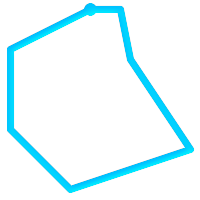 (c) |  (d) |
(a) and
(c) are simple
|
A MULTILINESTRING is simple
only if all of its elements are simple and the only intersection between
any two elements occurs at POINTs that are on the
boundaries of both elements.
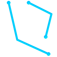 (e) |  (f) |  (g) |
(e) and
(f) are simple
|
By definition, a POLYGON is always
simple. It is valid if no two
rings in the boundary (made up of an exterior ring and interior rings)
cross. The boundary of a POLYGON may intersect at a
POINT but only as a tangent (i.e. not on a line).
A POLYGON may not have cut lines or spikes and the
interior rings must be contained entirely within the exterior ring.
 (h) |  (i) |  (j) |
 (k) |  (l) |  (m) |
(h) and
(i) are valid
|
A MULTIPOLYGON is valid
if and only if all of its elements are valid and the interiors of no two
elements intersect. The boundaries of any two elements may touch, but
only at a finite number of POINTs.
 (n) |  (o) |  (p) |
(n) and
(o) are not valid
|
Most of the functions implemented by the GEOS library rely on the assumption that your geometries are valid as specified by the OpenGIS Simple Feature Specification. To check simplicity or validity of geometries you can use the ST_IsSimple() and ST_IsValid()
-- Typically, it doesn't make sense to check
-- for validity on linear features since it will always return TRUE.
-- But in this example, PostGIS extends the definition of the OGC IsValid
-- by returning false if a LineString has less than 2 *distinct* vertices.
gisdb=# SELECT
   ST_IsValid('LINESTRING(0 0, 1 1)'),
   ST_IsValid('LINESTRING(0 0, 0 0, 0 0)');

 st_isvalid | st_isvalid
------------+-----------
      t     |     f
By default, PostGIS does not apply this validity check on geometry input, because testing for validity needs lots of CPU time for complex geometries, especially polygons. If you do not trust your data sources, you can manually enforce such a check to your tables by adding a check constraint:
ALTER TABLE mytable
  ADD CONSTRAINT geometry_valid_check
	CHECK (ST_IsValid(geom));
If you encounter any strange error messages such as "GEOS Intersection() threw an error!" when calling PostGIS functions with valid input geometries, you likely found an error in either PostGIS or one of the libraries it uses, and you should contact the PostGIS developers. The same is true if a PostGIS function returns an invalid geometry for valid input.
| |
The ST_IsValid() function does not check the Z and M dimensions. |
Once you have created a spatial table, you are ready to upload spatial data to the database. There are two built-in ways to get spatial data into a PostGIS/PostgreSQL database: using formatted SQL statements or using the Shapefile loader.
If spatial data can be converted to a text representation (as either WKT or WKB), then using
SQL might be the easiest way to get data into PostGIS.
Data can be bulk-loaded into PostGIS/PostgreSQL by loading a
text file of SQL INSERT statements using the psql SQL utility.
A SQL load file (roads.sql for example)
might look like this:
BEGIN;
INSERT INTO roads (road_id, roads_geom, road_name)
  VALUES (1,'LINESTRING(191232 243118,191108 243242)','Jeff Rd');
INSERT INTO roads (road_id, roads_geom, road_name)
  VALUES (2,'LINESTRING(189141 244158,189265 244817)','Geordie Rd');
INSERT INTO roads (road_id, roads_geom, road_name)
  VALUES (3,'LINESTRING(192783 228138,192612 229814)','Paul St');
INSERT INTO roads (road_id, roads_geom, road_name)
  VALUES (4,'LINESTRING(189412 252431,189631 259122)','Graeme Ave');
INSERT INTO roads (road_id, roads_geom, road_name)
  VALUES (5,'LINESTRING(190131 224148,190871 228134)','Phil Tce');
INSERT INTO roads (road_id, roads_geom, road_name)
  VALUES (6,'LINESTRING(198231 263418,198213 268322)','Dave Cres');
COMMIT;
The SQL file can be loaded into PostgreSQL using psql:
psql -d [database] -f roads.sql
The shp2pgsql data loader converts Shapefiles into SQL suitable for
insertion into a PostGIS/PostgreSQL database either in geometry or geography format.
The loader has several operating modes selected by command line flags.
There is also a shp2pgsql-gui graphical interface with most
of the options as the command-line loader.
This may be easier to use for one-off non-scripted loading or if you are new to PostGIS.
It can also be configured as a plugin to PgAdminIII.
- (c|a|d|p) These are mutually exclusive options:
- -c
Creates a new table and populates it from the Shapefile. This is the default mode.
- -a
Appends data from the Shapefile into the database table. Note that to use this option to load multiple files, the files must have the same attributes and same data types.
- -d
Drops the database table before creating a new table with the data in the Shapefile.
- -p
Only produces the table creation SQL code, without adding any actual data. This can be used if you need to completely separate the table creation and data loading steps.
- -?
Display help screen.
- -D
Use the PostgreSQL "dump" format for the output data. This can be combined with -a, -c and -d. It is much faster to load than the default "insert" SQL format. Use this for very large data sets.
- -s [<FROM_SRID>:]<SRID>
Creates and populates the geometry tables with the specified SRID. Optionally specifies that the input shapefile uses the given FROM_SRID, in which case the geometries will be reprojected to the target SRID.
- -k
Keep identifiers' case (column, schema and attributes). Note that attributes in Shapefile are all UPPERCASE.
- -i
Coerce all integers to standard 32-bit integers, do not create 64-bit bigints, even if the DBF header signature appears to warrant it.
- -I
Create a GiST index on the geometry column.
- -m
-m
a_file_nameSpecify a file containing a set of mappings of (long) column names to 10 character DBF column names. The content of the file is one or more lines of two names separated by white space and no trailing or leading space. For example:COLUMNNAME DBFFIELD1 AVERYLONGCOLUMNNAME DBFFIELD2
- -S
Generate simple geometries instead of MULTI geometries. Will only succeed if all the geometries are actually single (I.E. a MULTIPOLYGON with a single shell, or or a MULTIPOINT with a single vertex).
- -t <dimensionality>
Force the output geometry to have the specified dimensionality. Use the following strings to indicate the dimensionality: 2D, 3DZ, 3DM, 4D.
If the input has fewer dimensions that specified, the output will have those dimensions filled in with zeroes. If the input has more dimensions that specified, the unwanted dimensions will be stripped.
- -w
Output WKT format, instead of WKB. Note that this can introduce coordinate drifts due to loss of precision.
- -e
Execute each statement on its own, without using a transaction. This allows loading of the majority of good data when there are some bad geometries that generate errors. Note that this cannot be used with the -D flag as the "dump" format always uses a transaction.
- -W <encoding>
Specify encoding of the input data (dbf file). When used, all attributes of the dbf are converted from the specified encoding to UTF8. The resulting SQL output will contain a
SET CLIENT_ENCODING to UTF8command, so that the backend will be able to reconvert from UTF8 to whatever encoding the database is configured to use internally.- -N <policy>
NULL geometries handling policy (insert*,skip,abort)
- -n
-n Only import DBF file. If your data has no corresponding shapefile, it will automatically switch to this mode and load just the dbf. So setting this flag is only needed if you have a full shapefile set, and you only want the attribute data and no geometry.
- -G
Use geography type instead of geometry (requires lon/lat data) in WGS84 long lat (SRID=4326)
- -T <tablespace>
Specify the tablespace for the new table. Indexes will still use the default tablespace unless the -X parameter is also used. The PostgreSQL documentation has a good description on when to use custom tablespaces.
- -X <tablespace>
Specify the tablespace for the new table's indexes. This applies to the primary key index, and the GIST spatial index if -I is also used.
- -Z
When used, this flag will prevent the generation of
ANALYZEstatements. Without the -Z flag (default behavior), theANALYZEstatements will be generated.
An example session using the loader to create an input file and loading it might look like this:
# shp2pgsql -c -D -s 4269 -i -I shaperoads.shp myschema.roadstable > roads.sql
# psql -d roadsdb -f roads.sql
A conversion and load can be done in one step using UNIX pipes:
# shp2pgsql shaperoads.shp myschema.roadstable | psql -d roadsdb
Spatial data can be extracted from the database using either SQL or the Shapefile dumper. The section on SQL presents some of the functions available to do comparisons and queries on spatial tables.
The most straightforward way of extracting spatial data out of the
database is to use a SQL SELECT query
to define the data set to be extracted
and dump the resulting columns into a parsable text file:
db=# SELECT road_id, ST_AsText(road_geom) AS geom, road_name FROM roads;

road_id | geom                                    | road_name
--------+-----------------------------------------+-----------
	  1 | LINESTRING(191232 243118,191108 243242) | Jeff Rd
	  2 | LINESTRING(189141 244158,189265 244817) | Geordie Rd
	  3 | LINESTRING(192783 228138,192612 229814) | Paul St
	  4 | LINESTRING(189412 252431,189631 259122) | Graeme Ave
	  5 | LINESTRING(190131 224148,190871 228134) | Phil Tce
	  6 | LINESTRING(198231 263418,198213 268322) | Dave Cres
	  7 | LINESTRING(218421 284121,224123 241231) | Chris Way
(6 rows)
There will be times when some kind of restriction is necessary to cut down the number of records returned. In the case of attribute-based restrictions, use the same SQL syntax as used with a non-spatial table. In the case of spatial restrictions, the following functions are useful:
- ST_Intersects
This function tells whether two geometries share any space.
- =
This tests whether two geometries are geometrically identical. For example, if 'POLYGON((0 0,1 1,1 0,0 0))' is the same as 'POLYGON((0 0,1 1,1 0,0 0))' (it is).
Next, you can use these operators in queries. Note that when specifying geometries and boxes on the SQL command line, you must explicitly turn the string representations into geometries function. The 312 is a fictitious spatial reference system that matches our data. So, for example:
SELECT road_id, road_name
  FROM roads
  WHERE roads_geom='SRID=312;LINESTRING(191232 243118,191108 243242)'::geometry;
The above query would return the single record from the "ROADS_GEOM" table in which the geometry was equal to that value.
To check whether some of the roads passes in the area defined by a polygon:
SELECT road_id, road_name
FROM roads
WHERE ST_Intersects(roads_geom, 'SRID=312;POLYGON((...))');
The most common spatial query will probably be a "frame-based" query, used by client software, like data browsers and web mappers, to grab a "map frame" worth of data for display.
When using the "&&" operator, you can specify either a BOX3D as the comparison feature or a GEOMETRY. When you specify a GEOMETRY, however, its bounding box will be used for the comparison.
Using a "BOX3D" object for the frame, such a query looks like this:
SELECT ST_AsText(roads_geom) AS geom
FROM roads
WHERE
  roads_geom && ST_MakeEnvelope(191232, 243117,191232, 243119,312);
Note the use of the SRID 312, to specify the projection of the envelope.
The pgsql2shp table dumper connects
to the database and converts a table (possibly defined by a query) into
a shape file. The basic syntax is:
pgsql2shp [<options>] <database> [<schema>.]<table>
pgsql2shp [<options>] <database> <query>
The commandline options are:
- -f <filename>
Write the output to a particular filename.
- -h <host>
The database host to connect to.
- -p <port>
The port to connect to on the database host.
- -P <password>
The password to use when connecting to the database.
- -u <user>
The username to use when connecting to the database.
- -g <geometry column>
In the case of tables with multiple geometry columns, the geometry column to use when writing the shape file.
- -b
Use a binary cursor. This will make the operation faster, but will not work if any NON-geometry attribute in the table lacks a cast to text.
- -r
Raw mode. Do not drop the
gidfield, or escape column names.- -m
filename Remap identifiers to ten character names. The content of the file is lines of two symbols separated by a single white space and no trailing or leading space: VERYLONGSYMBOL SHORTONE ANOTHERVERYLONGSYMBOL SHORTER etc.
Spatial indexes make using a spatial database for large data sets possible. Without indexing, a search for features requires a sequential scan of every record in the database. Indexing speeds up searching by organizing the data into a structure which can be quickly traversed to find matching records.
The B-tree index method commonly used for attribute data is not very useful for spatial data, since it only supports storing and querying data in a single dimension. Data such as geometry (which has 2 or more dimensions) requires an index method that supports range query across all the data dimensions. One of the key advantages of PostgreSQL for spatial data handling is that it offers several kinds of index methods which work well for multi-dimensional data: GiST, BRIN and SP-GiST indexes.
GiST (Generalized Search Tree) indexes break up data into "things to one side", "things which overlap", "things which are inside" and can be used on a wide range of data-types, including GIS data. PostGIS uses an R-Tree index implemented on top of GiST to index spatial data. GiST is the most commonly-used and versatile spatial index method, and offers very good query performance.
BRIN (Block Range Index) indexes operate by summarizing the spatial extent of ranges of table records. Search is done via a scan of the ranges. BRIN is only appropriate for use for some kinds of data (spatially sorted, with infrequent or no update). But it provides much faster index create time, and much smaller index size.
SP-GiST (Space-Partitioned Generalized Search Tree) is a generic index method that supports partitioned search trees such as quad-trees, k-d trees, and radix trees (tries).
Spatial indexes store only the bounding box of geometries. Spatial queries use the index as a primary filter to quickly determine a set of geometries potentially matching the query condition. Most spatial queries require a secondary filter that uses a spatial predicate function to test a more specific spatial condition. For more information on queying with spatial predicates see Section 5.2, “Using Spatial Indexes”.
See also the PostGIS Workshop section on spatial indexes, and the PostgreSQL manual.
GiST stands for "Generalized Search Tree" and is a generic form of indexing for multi-dimensional data. PostGIS uses an R-Tree index implemented on top of GiST to index spatial data. GiST is the most commonly-used and versatile spatial index method, and offers very good query performance. Other implementations of GiST are used to speed up searches on all kinds of irregular data structures (integer arrays, spectral data, etc) which are not amenable to normal B-Tree indexing. For more information see the PostgreSQL manual.
Once a spatial data table exceeds a few thousand rows, you will want to build an index to speed up spatial searches of the data (unless all your searches are based on attributes, in which case you'll want to build a normal index on the attribute fields).
The syntax for building a GiST index on a "geometry" column is as follows:
CREATE INDEX [indexname] ON [tablename] USING GIST ( [geometryfield] );
The above syntax will always build a 2D-index. To get the an n-dimensional index for the geometry type, you can create one using this syntax:
CREATE INDEX [indexname] ON [tablename] USING GIST ([geometryfield] gist_geometry_ops_nd);
Building a spatial index is a computationally intensive exercise. It also blocks write access to your table for the time it creates, so on a production system you may want to do in in a slower CONCURRENTLY-aware way:
CREATE INDEX CONCURRENTLY [indexname] ON [tablename] USING GIST ( [geometryfield] );
After building an index, it is sometimes helpful to force PostgreSQL to collect table statistics, which are used to optimize query plans:
VACUUM ANALYZE [table_name] [(column_name)];
BRIN stands for "Block Range Index". It is a general-purpose index method introduced in PostgreSQL 9.5. BRIN is a lossy index method, meaning that a secondary check is required to confirm that a record matches a given search condition (which is the case for all provided spatial indexes). It provides much faster index creation and much smaller index size, with reasonable read performance. Its primary purpose is to support indexing very large tables on columns which have a correlation with their physical location within the table. In addition to spatial indexing, BRIN can speed up searches on various kinds of attribute data structures (integer, arrays etc). For more information see the PostgreSQL manual.
Once a spatial table exceeds a few thousand rows, you will want to build an index to speed up spatial searches of the data. GiST indexes are very performant as long as their size doesn't exceed the amount of RAM available for the database, and as long as you can afford the index storage size, and the cost of index update on write. Otherwise, for very large tables BRIN index can be considered as an alternative.
A BRIN index stores the bounding box enclosing all the geometries contained in the rows in a contiguous set of table blocks, called a block range. When executing a query using the index the block ranges are scanned to find the ones that intersect the query extent. This is efficient only if the data is physically ordered so that the bounding boxes for block ranges have minimal overlap (and ideally are mutually exclusive). The resulting index is very small in size, but is typically less performant for read than a GiST index over the same data.
Building a BRIN index is much less CPU-intensive than building a GiST index. It's common to find that a BRIN index is ten times faster to build than a GiST index over the same data. And because a BRIN index stores only one bounding box for each range of table blocks, it's common to use up to a thousand times less disk space than a GiST index.
You can choose the number of blocks to summarize in a range. If you decrease this number, the index will be bigger but will probably provide better performance.
For BRIN to be effective, the table data should be stored in a physical order which minimizes the amount of block extent overlap. It may be that the data is already sorted appropriately (for instance, if it is loaded from another dataset that is already sorted in spatial order). Otherwise, this can be accomplished by sorting the data by a one-dimensional spatial key. One way to do this is to create a new table sorted by the geometry values (which in recent PostGIS versions uses an efficient Hilbert curve ordering):
CREATE TABLE table_sorted AS
   SELECT * FROM table  ORDER BY geom;
Alternatively, data can be sorted in-place by using a GeoHash as a (temporary) index, and clustering on that index:
CREATE INDEX idx_temp_geohash ON table
    USING btree (ST_GeoHash( ST_Transform( geom, 4326 ), 20));
CLUSTER table USING idx_temp_geohash;
The syntax for building a BRIN index on a geometry column is:
CREATE INDEX [indexname] ON [tablename] USING BRIN ( [geome_col] );
The above syntax builds a 2D index. To build a 3D-dimensional index, use this syntax:
CREATE INDEX [indexname] ON [tablename]
    USING BRIN ([geome_col] brin_geometry_inclusion_ops_3d);
You can also get a 4D-dimensional index using the 4D operator class:
CREATE INDEX [indexname] ON [tablename]
    USING BRIN ([geome_col] brin_geometry_inclusion_ops_4d);
The above commands use the default number of blocks in a range, which is 128. To specify the number of blocks to summarise in a range, use this syntax
CREATE INDEX [indexname] ON [tablename]
    USING BRIN ( [geome_col] ) WITH (pages_per_range = [number]);
Keep in mind that a BRIN index only stores one index entry for a large number of rows. If your table stores geometries with a mixed number of dimensions, it's likely that the resulting index will have poor performance. You can avoid this performance penalty by choosing the operator class with the least number of dimensions of the stored geometries
The geography datatype is supported for BRIN indexing. The
syntax for building a BRIN index on a geography column is:
CREATE INDEX [indexname] ON [tablename] USING BRIN ( [geog_col] );
The above syntax builds a 2D-index for geospatial objects on the spheroid.
Currently, only "inclusion support" is provided, meaning
that just the &&, ~ and
@ operators can be used for the 2D cases (for both
geometry and geography), and just the &&&
operator for 3D geometries.
There is currently no support for kNN searches.
An important difference between BRIN and other index types is that the database does not
maintain the index dynamically. Changes to spatial data in the table
are simply appended to the end of the index. This will cause index search performance to
degrade over time. The index can be updated by performing a VACUUM,
or by using a special function brin_summarize_new_values(regclass).
For this reason BRIN may be most appropriate for use with data that is read-only,
or only rarely changing. For more information refer to the
manual.
To summarize using BRIN for spatial data:
Index build time is very fast, and index size is very small.
Index query time is slower than GiST, but can still be very acceptable.
Requires table data to be sorted in a spatial ordering.
Requires manual index maintenance.
Most appropriate for very large tables, with low or no overlap (e.g. points), which are static or change infrequently.
More effective for queries which return relatively large numbers of data records.
SP-GiST stands for "Space-Partitioned Generalized Search Tree" and is a generic form of indexing for multi-dimensional data types that supports partitioned search trees, such as quad-trees, k-d trees, and radix trees (tries). The common feature of these data structures is that they repeatedly divide the search space into partitions that need not be of equal size. In addition to spatial indexing, SP-GiST is used to speed up searches on many kinds of data, such as phone routing, ip routing, substring search, etc. For more information see the PostgreSQL manual.
As it is the case for GiST indexes, SP-GiST indexes are lossy, in the sense that they store the bounding box enclosing spatial objects. SP-GiST indexes can be considered as an alternative to GiST indexes.
Once a GIS data table exceeds a few thousand rows, an SP-GiST index may be used to speed up spatial searches of the data. The syntax for building an SP-GiST index on a "geometry" column is as follows:
CREATE INDEX [indexname] ON [tablename] USING SPGIST ( [geometryfield] );
The above syntax will build a 2-dimensional index. A 3-dimensional index for the geometry type can be created using the 3D operator class:
CREATE INDEX [indexname] ON [tablename] USING SPGIST ([geometryfield] spgist_geometry_ops_3d);
Building a spatial index is a computationally intensive operation. It also blocks write access to your table for the time it creates, so on a production system you may want to do in in a slower CONCURRENTLY-aware way:
CREATE INDEX CONCURRENTLY [indexname] ON [tablename] USING SPGIST ( [geometryfield] );
After building an index, it is sometimes helpful to force PostgreSQL to collect table statistics, which are used to optimize query plans:
VACUUM ANALYZE [table_name] [(column_name)];
An SP-GiST index can accelerate queries involving the following operators:
<<, &<, &>, >>, <<|, &<|, |&>, |>>, &&, @>, <@, and ~=, for 2-dimensional indexes,
&/&, ~==, @>>, and <<@, for 3-dimensional indexes.
There is no support for kNN searches at the moment.
Ordinarily, indexes invisibly speed up data access: once an index is built, the PostgreSQL query planner automatically decides when to use it to improve query performance. But there are some situations where the planner does not choose to use existing indexes, so queries end up using slow sequential scans instead of a spatial index.
If you find your spatial indexes are not being used, there are a few things you can do:
Examine the query plan and check your query actually computes the thing you need. An erroneous JOIN, either forgotten or to the wrong table, can unexpectedly retrieve table records multiple times. To get the query plan, execute with
EXPLAINin front of the query.Make sure statistics are gathered about the number and distributions of values in a table, to provide the query planner with better information to make decisions around index usage. VACUUM ANALYZE will compute both.
You should regularly vacuum your databases anyways. Many PostgreSQL DBAs run VACUUM as an off-peak cron job on a regular basis.
If vacuuming does not help, you can temporarily force the planner to use the index information by using the command SET ENABLE_SEQSCAN TO OFF;. This way you can check whether the planner is at all able to generate an index-accelerated query plan for your query. You should only use this command for debugging; generally speaking, the planner knows better than you do about when to use indexes. Once you have run your query, do not forget to run SET ENABLE_SEQSCAN TO ON; so that the planner will operate normally for other queries.
If SET ENABLE_SEQSCAN TO OFF; helps your query to run faster, your Postgres is likely not tuned for your hardware. If you find the planner wrong about the cost of sequential versus index scans try reducing the value of
RANDOM_PAGE_COSTinpostgresql.conf, or use SET RANDOM_PAGE_COST TO 1.1;. The default value forRANDOM_PAGE_COSTis 4.0. Try setting it to 1.1 (for SSD) or 2.0 (for fast magnetic disks). Decreasing the value makes the planner more likely to use index scans.If SET ENABLE_SEQSCAN TO OFF; does not help your query, the query may be using a SQL construct that the Postgres planner is not yet able to optimize. It may be possible to rewrite the query in a way that the planner is able to handle. For example, a subquery with an inline SELECT may not produce an efficient plan, but could possibly be rewritten using a LATERAL JOIN.
For more information see the Postgres manual section on Query Planning.