30. Rasters
PostGIS supports another kind of spatial data type called a raster. Raster data, much like geometry data, uses Cartesian coordinates and a spatial reference system. However instead of vector data, raster data is represented as an n-dimensional matrix consisting of pixels and bands. The bands defines the number of matrices you have. Each pixel stores a value corresponding to each band. So a 3-banded raster such as an RGB image, would have 3 values for each pixel corresponding to the Red-Green-Blue bands.
Although pretty pictures such as those you see on your TV screen are rasters, rasters may not be that exciting to look at. In a nutshell, a raster is a matrix, pinned on a coordinate system, that has values that can represent anything you want them to represent.
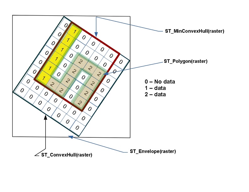
Since rasters live in cartesian space, rasters can interact with geometries. PostGIS offers many functions that take as input both rasters and geometries. Many operations applied to rasters will result in geometries. Common ones are the ST_Polygon, ST_Envelope, ST_ConvexHull, and ST_MinConvexHull as shown below. When you cast a raster to a geometry, what is output is the ST_ConvexHull of the raster.
The raster format is commonly used to store elevation data, temperature data, satellite data, and thematic data representing things like environmental contamination, population density, and environmental hazard occurrences. You can use rasters to store any numeric data that has a meaningful coordinate location. The only restriction is that for all data in a specific band the numeric data types have to be the same.
Although raster data can be created from scratch in PostGIS, a more common approach is to load raster data from various formats using the raster2pgsql command line tool packaged with PostGIS. Before all of that, you must enable raster support in your database by running the command:
CREATE EXTENSION postgis_raster;
30.1. Creating Rasters From Geometries
We’ll start off by first creating raster data from vector data, and then move on to the more exciting approach of loading data from a raster source. You will find that raster data is available in abundance and often free from various government sites.
We’ll start by converting some geometries into rasters using ST_AsRaster function as follows.
CREATE TABLE rasters (name varchar, rast raster);

INSERT INTO rasters(name, rast)
SELECT f.word, ST_AsRaster(geom, width=>150, height=>150)
FROM (VALUES ('Hello'), ('Raster') ) AS f(word)
  , ST_Letters(word) AS geom;

CREATE INDEX ix_rasters_rast
  ON rasters USING gist(ST_ConvexHull(rast));
The above example CREATEs a table (rasters) from geometries formed from letters using the PostGIS 3.2+ ST_Letters function. Rasters similar to geometries, can take advantage of spatial indexes. The spatial index used for raster is a functional index that indexes the geometry convexhull of the raster.
You can see some useful metadata of your rasters with the following query which utilizes the postgis raster ST_Count function to count the number of pixels that have data and the ST_MetaData function to provide all sorts of useful background info for our rasters.
SELECT name, ST_Count(rast) As num_pixels, md.*
   FROM rasters, ST_MetaData(rast) AS md;
name  | num_pixels | upperleftx |    upperlefty     | width | height |       scalex       |       scaley        | skewx | skewy | srid | numbands
--------+------------+------------+-------------------+-------+--------+--------------------+---------------------+-------+-------+------+----------
Hello  |      13926 |          0 | 77.10000000000001 |   150 |    150 |  1.226888888888889 | -0.5173333333333334 |     0 |     0 |    0 |        1
Raster |      11967 |          0 |              75.4 |   150 |    150 | 1.7226319023207244 | -0.5086666666666667 |     0 |     0 |    0 |        1
(2 rows)
Note
There are two levels of raster functions. There are functions such as ST_MetaData that work at the raster level and there are functions such as ST_Count function and ST_BandMetaData function that work at the band level. Most functions in postgis raster that work at the band level, work with only one band at a time, and assume the band you want is 1.
If you have a multi-band raster, and you need to count the pixel not no-data values in a band other than 1, you would explicitly specify the band number as follows ST_Count(rast,2).
Note how all the rasters have a 150x150 dimension. This is not ideal. This means that in order to force that, our rasters, are squished in all sorts of ways. If only we could see the ugliness of the rasters before us.
30.2. Loading Rasters using raster2pgsql
raster2pgsql is a command-line tool often packaged with PostGIS.
If you are on windows and used application stackbuilder PostGIS Bundle, you’ll find raster2pgsql.exe in the folder C:\Program Files\PostgreSQL\15\bin where the 15 should be replaced with the version of PostgreSQL you are running.
If you are using Postgres.App, you’ll find raster2pgsql among the other Postgres.app CLI Tools.
On Ubuntu and Debian, you will need
apt install postgis
to have the PostGIS commandline tools installed. This may install an additional version of PostgreSQL as well. You can see a list of clusters in Debian/Ubuntu using the pg_lsclusters command and drop them using the pg_dropcluster command.
For this and later exercises, we’ll be using nyc_dem.tif found in the file PG Raster Workshop Dataset https://postgis.net/stuff/workshop-data/postgis_raster_workshop.zip. For some geometry/raster examples, we will also be using NYC data loaded from prior chapters. In-lieu of loading the tif, you can restore the nyc_dem.backup included in the zip file in your database using the pg_restore commandline tool or the pgAdmin Restore menu.
Note
This raster data was sourced from NYC DEM 1-foot Integer which is a 3GB DEM tif representing elevation relative to sea level with buildings and overwater removed. We then created a lower res version of it.
The raster2pgsql tool is similar to the shp2gpsql except instead of loading ESRI shapefiles into PostGIS geometry/geography tables, it loads any GDAL supported raster format into raster tables. Just like shp2pgsql you can pass it a spatial reference id (SRID) of the source. Unlike shp2pgsql it can infer the spatial references system of the source data if your source data has suitable metadata.
For a full exposure of all the possible switches offered refer to raster2pgsql options.
Some other notable options raster2pgsql offers which we will not cover are:
Ability to denote the SRID of the source. Instead, we’ll rely on raster2pgsql guessing skills.
Ability to set the nodata value, when not specified, raster2pgsql tries to infer from the file.
Abiliity to load out-of-database rasters.
To load all the tif files in our folder and also create overviews, we would run the below.
raster2pgsql -d -e -l 2,3 -I -C -M -F -Y -t 256x256 *.tif nyc_dem | psql -d nyc
-d to drop the tables if they already exist
The above command uses -e to do load immediately instead of committing in a transaction
-C set raster constraints, this is useful for raster_columns to show info. You may want to combine with -x to exclude the extent constraint, which is a slow constraint to check and also hampers future loads in the table.
-M to vacuum and analyze after load, to improve query planner statistics
-Y to use copy in batches of 50. If you are running PostGIS 3.3 or higher, you can use -Y 1000 to have copy be in batches of 1000, or even higher number. This will run faster, but will use more memory.
-l 2,3 to create over view tables: o_2_ncy_dem and o_3_nyc_dem. This is useful for viewing data.
-I to create a spatial index
-F to add file name, if you have only one tif file, this is kinda pointless. If you had multiple, this would be useful to tell you what file each row came from.
-t to set the block size. Note if you are not sure the best size use, use -t auto instead and raster2pgql will use the same tiling as what was in the tif. The output will tell you what the blocksize is it chose. Cancel if it looks huge or weird. The original file had a size of 300x7 which is not ideal.
Use psql to run the generated sql against the database. If you want to dump to a file instead, use > nyc_dem.sql
For this example, we have only one tif file, so we could instead specify the full file name, instead of *.tif. If the files are not in your current directory, you can also specify a folder path with *.tif.
Note
If you are on windows and need to reference the folder, make sure to include the drive letter such as C:/workshop/*.tif
You’ll often hear in PostGIS lingo, the term raster tile and raster used somewhat interchangeably. A raster tile really corresponds to a particular raster in a raster column which is a subset of a bigger raster, such as this NYC dem data we just loaded. This is because when rasters are loaded into PostGIS from big raster files, they chopped into many rows to make them manageable. Each raster in each row then is a part of a bigger raster. Each tile covers same size area denoted by the blocksize you specified. Rasters are sadly limited by the 1GB PostgreSQL TOAST limit and also the slow process of detoasting and so we need to chop up in order to achieve decent performance or to even store them.
30.3. Viewing Rasters in Browser
Although pgAdmin and psql have no mechanism yet to view postgis rasters, we have a couple of options. For smallish rasters the easiest is to output to a web-friendly raster format such as PNG using batteries included postgis raster functions like ST_AsPNG or ST_AsGDALRaster listed in PostGIS Raster output functions. As your rasters get larger, you’ll want to graduate to a tool such as QGIS to view them in all their glory or the GDAL family of commandline tools such as gdal_translate to export them to other raster formats. Remember though, postgis rasters are built for analysis, not for generating pretty pictures for you to look at.
One caveat, by default all different raster types outputs are disabled. In order to utilize these, you’ll need to enable drivers, all or a subset as detailed in Enable GDAL Raster drivers
SET postgis.gdal_enabled_drivers = 'ENABLE_ALL';
If you don’t want to have to do this for each connection, you can set at the database level using:
ALTER DATABASE nyc SET postgis.gdal_enabled_drivers = 'ENABLE_ALL';
Each new connection to the database will use that setting.
Run the below query and copy and paste the output into the address bar of your web browser.
SELECT 'data:image/png;base64,' ||
   encode(ST_AsPNG(rast),'base64')
   FROM rasters
   WHERE name = 'Hello';

For the rasters created thus far, we didn’t specify the number of bands nor did we even define their relation to earth. As such our rasters have an unknown spatial reference system (0).
You can think of a rasters exoskeletal as a geometry. A matrix encased in a geometric envelop. In order to do useful analysis, we need to georeference our rasters, meaning we want each pixel (rectangle) to represent some meaningful plot of space.
The ST_AsRaster has many overloaded representations. The earlier example used the simplest such implementation and accepted the default arguments which are 8BUI and 1 band, with no data being 0. If you need to use the other variants, you should use the named arguments call syntax so that you don’t accidentally fall into the wrong variant of the function or get function is not unique errors.
If you start with a geometry that has a spatial reference system, you’ll end up with a raster with same spatial reference system. In this next example, we’ll plop our words in New York in bright cheery colors. We will also use pixel scale instead of width and height so that our raster pixel sizes represent 1 meter x 1 meter of space.
INSERT INTO rasters(name, rast)
SELECT f.word || ' in New York' ,
  ST_AsRaster(geom,
    scalex => 1.0, scaley => -1.0,
    pixeltype => ARRAY['8BUI', '8BUI', '8BUI'],
    value => CASE WHEN word = 'Hello' THEN
      ARRAY[10,10,100] ELSE ARRAY[10,100,10] END,
    nodataval => ARRAY[0,0,0], gridx => NULL, gridy => NULL
    ) AS rast
FROM (
    VALUES ('Hello'), ('Raster') ) AS f(word)
  , ST_SetSRID(
      ST_Translate(ST_Letters(word),586467,4504725), 26918
    ) AS geom;
If we then look at this, we’ll see a non-squashed colored geometry.
SELECT 'data:image/png;base64,' ||
   encode(ST_AsPNG(rast),'base64')
   FROM rasters
   WHERE name = 'Hello in New York';

Repeat for Raster:
SELECT 'data:image/png;base64,' ||
   encode(ST_AsPNG(rast),'base64')
   FROM rasters
   WHERE name = 'Raster in New York';

What is more telling, if we rerun the
SELECT name, ST_Count(rast) As num_pixels, md.*
  FROM rasters, ST_MetaData(rast) AS md;
Observe the metadata of the New York entries. They have the New York state plane meter spatial reference system. They also have the same scale. Since each unit is 1x1 meter, the width of the word Raster is now wider than Hello.
      name         | num_pixels | upperleftx |    upperlefty     | width | height |       scalex       |       scaley        | skewx | skewy | srid  | numbands
-------------------+------------+------------+-------------------+-------+--------+--------------------+---------------------+-------+-------+-------+----------
Hello              |      13926 |          0 | 77.10000000000001 |   150 |    150 |  1.226888888888889 | -0.5173333333333334 |     0 |     0 |     0 |        1
Raster             |      11967 |          0 |              75.4 |   150 |    150 | 1.7226319023207244 | -0.5086666666666667 |     0 |     0 |     0 |        1
Hello in New York  |       8786 |     586467 |         4504802.1 |   184 |     78 |                  1 |                  -1 |     0 |     0 | 26918 |        3
Raster in New York |      10544 |     586467 |         4504800.4 |   258 |     76 |                  1 |                  -1 |     0 |     0 | 26918 |        3
(4 rows)
30.4. Raster Spatial Catalog tables
Similar to the geometry and geography types, raster has a set of catalogs that show you all raster columns in your database. These are raster_columns and raster_overviews.
30.4.1. raster_columns
The raster_columns view to the sibling to the geometry_columns and geography_columns, providing much the same data and more, but for raster columns.
SELECT *
    FROM raster_columns;
Explore the table, and you’ll find this:
r_table_catalog | r_table_schema | r_table_name | r_raster_column | srid | scale_x | scale_y | blocksize_x | blocksize_y | same_alignment | regular_blocking | num_bands | pixel_types | nodata_values | out_db | extent | spatial_index
----------------+----------------+--------------+-----------------+------+---------+---------+-------------+-------------+----------------+------------------+-----------+-------------+---------------+--------+--------+---------------
nyc             | public         | rasters      | rast            |    0 |         |         |             |             | f              | f                |           |             |               |        |        | t
nyc             | public         | nyc_dem      | rast            | 2263 |      10 |     -10 |         256 |         256 | t              | f                |         1 | {16BUI}     | {NULL}        | {f}    |        | t
nyc             | public         | o_2_nyc_dem  | rast            | 2263 |      20 |     -20 |         256 |         256 | t              | f                |         1 | {16BUI}     | {NULL}        | {f}    |        | t
nyc             | public         | o_3_nyc_dem  | rast            | 2263 |      30 |     -30 |         256 |         256 | t              | f                |         1 | {16BUI}     | {NULL}        | {f}    |        | t
(4 rows)
a disappointing row of largely unfilled information for the rasters table.
Unlike geometry and geography, raster does not support type modifiers, because type modifier space is too limited and there are more critical properties than what can fit in a type modifier.
Raster instead relies on constraints, and reads these constraints back as part of the view.
Look at the other rows from the tables we loaded using raster2pgsql. Because we used the -C switch raster2pgsql added constraints for the srid and other info it was able to read from the tif or that we passed in. The overview tables generated with the -l switch o_2_nyc_dem and o_3_nyc_dem show up as well.
Let’s try to add some constraints to our table.
SELECT AddRasterConstraints('public'::name, 'rasters'::name, 'rast'::name);
And you’ll be bombarded with a whole bunch of notices about how your raster data is a mess and nothing can be constrained. If you look at raster_columns again, still the same disappointing story of many blank rows for rasters.
In order for constraints to be applied, all rasters in your table must be constrainable by at least one rule.
We can perhaps do this, let’s just lie and say all our data is in New York State plane.
UPDATE rasters SET rast = ST_SetSRID(rast,26918)
  WHERE ST_SRID(rast) <> 26918;

SELECT AddRasterConstraints('public'::name, 'rasters'::name, 'rast'::name);
SELECT r_table_name AS t, r_raster_column AS c, srid,
  blocksize_x AS bx, blocksize_y AS by, scale_x AS sx, scale_y AS sy,
  ST_AsText(extent) AS e
  FROM raster_columns
WHERE r_table_name = 'rasters';
Ah progress:
t         |  c   | srid  | bx  | by  | sx | sy |  e
----------+------+-------+-----+-----+----+----+------------------------------------------
rasters   | rast | 26918 | 150 | 150 |    |    | POLYGON((0 -0.90000000000..
(1 row)
The more you can constrain all your rasters, the more columns you’ll see filled in and also the more operations you’ll be able to do across all the tiles in your raster. Keep in mind that in some cases, you may not want to apply all constraints.
For example, if you plan to load more data into your raster table, you’ll want to skip the extent constraint since that would require that all rasters are within the extent of the extent constraint.
30.4.2. raster_overviews
Raster overview columns appear both in the raster_columns meta catalog and another meta catalog called raster_overviews. Overviews are used mostly to speed up viewing at higher zoom levels. They can also be used for quick back of the envelop analysis, providing less accurate stats, but at a much faster speed than applying to the raw raster table.
To inspect the overviews, run:
SELECT *
    FROM raster_overviews;
and you’ll see the output:
o_table_catalog | o_table_schema | o_table_name | o_raster_column | r_table_catalog | r_table_schema | r_table_name | r_raster_column | overview_factor
----------------+----------------+--------------+-----------------+-----------------+----------------+--------------+-----------------+-----------------
nyc             | public         | o_2_nyc_dem  | rast            | nyc             | public         | nyc_dem      | rast            |               2
nyc             | public         | o_3_nyc_dem  | rast            | nyc             | public         | nyc_dem      | rast            |               3
(2 rows)
The raster_overviews table only provides you the overview_factor and the name of the parent table. All this information is something you could have figured out yourself by the raster2pgsql naming convention for overviews.
The overview_factor tells you at what resolution the row is with respect to it’s parent. An overview_factor of 2 means that 2x2 = 4 tiles can fit into one overview_2 tile. Similarly an overview_factor of 3 meants that 2x2x2 = 8 tiles of the original can be shoved into an overview_3 tile.
30.5. Common Raster Functions
The postgis_raster extension has over 100 functions to choose from. PostGIS raster functionality was patterned after the PostGIS geometry support. You’ll find an overlap of functions between raster and geometry where it makes sense. Common ones you’ll use that have equivalent in geometry world are ST_Intersects, ST_SetSRID, ST_SRID, ST_Union, ST_Intersection, and ST_Transform.
In addition to those overlapping functions, it supports the && overlap operator between rasters and between a raster and geometry. It also offers many functions that work in conjunction with geometry or are very specific to rasters.
You need a function like ST_Union to reconstitute a region. Because performance gets slow, the more pixels a function needs to analyse, you need a fast acting function ST_Clip to clip the rasters to just the portions of interest for your analysis.
Finally you need ST_Intersects or && to zoom in on the raster tiles that contain your areas of interest. The && operator, is a faster process than the ST_Intersects. Both can take advantage of raster spatial indexes. We’ll cover these bread and butter functions first before moving on to other sections where we will use them in concert with other raster and geometry functions.
30.5.1. Unioning Rasters with ST_Union
The ST_Union function for raster, just as the geometry equivalent ST_Union, aggregates a set of rasters together into a single raster. However, just as with geometry, not all rasters can be combined together, but the rules for raster unioning are more complicated than geometry rules. In the case of geometries, all you need is to have the same spatial reference system, but for rasters that is not sufficient.
If you were to attempt, the following:
SELECT ST_Union(rast)
    FROM rasters;
You’d be summarily punished with an error:
ERROR: rt_raster_from_two_rasters: The two rasters provided do not have the same alignment SQL state: XX000
What is this same alignment thing, that is preventing you from unioning your precious rasters?
In order for rasters to be combined, they need to be on the same grid so to speak. Meaning they must have same pixel sizes, same orientation (the skew), same spatial reference system, and their pixels must not cut into each other, meaning they share the same worldly pixel grid.
If you try the same query, but just with words we carefully placed in New York.
Again, the same error. These are the same spatial ref system, the same pixel sizes, and yet it’s still not good enough. Because their grids are off.
We can fix this by shifting the upper left y coordinates ever so slightly and then trying again. If our grids start at integer level since our pixel sizes are whole integer, then the pixels won’t cut into each other.
UPDATE rasters SET rast = ST_SetUpperLeft(rast,
  ST_UpperLeftX(rast)::integer,
  ST_UpperLeftY(rast)::integer)
WHERE name LIKE '%New York';

SELECT ST_Union(rast ORDER BY name)
  FROM rasters
  WHERE name LIKE '%New York%';
Voila it worked, and if we were to view, we’d see something like this:

Note
If ever you are unclear why your rasters don’t have the same alignment, you can use the function ST_SameAlignment, which will compare 2 rasters or a set of rasters and tell you if they have the same alignment. If you have notices enabled, the NOTICE will tell you what is off with the rasters in question. The ST_NotSameAlignmentReason, instead of just a notice will output the reason. It however only works with two rasters at a time.
One major way in which the ST_Union(raster) raster function deviates from the ST_Union(geometry) geometry function is that it allows for an argument called uniontype. This argument by default is set to LAST if you don’t specify it, which means, take the LAST raster pixel values in occasions where the raster pixel values overlap. As a general rule, pixels in a band that are marked as no-data are ignored.
Just as with most aggregates in PostgreSQL, you can put a ORDER BY clause as part of the function call as is done in the prior example. Specifying the order, allows you to control which raster takes priority. So in our prior example, Raster trumped Hello because Raster is alphabetically last.
Observe, if you switch the order:
SELECT ST_Union(rast ORDER BY name DESC)
  FROM rasters
  WHERE name LIKE '%New York%';

Then Hello trumps Raster because Hello is now the last overlaid.
The FIRST union type is the reverse of LAST.
But on occassion, LAST may not be the right operation. Let’s suppose our rasters represented two different sets of observations from two different devices. These devices measure the same thing, and we aren’t sure which is right when they cross paths, so we’d instead like to take the MEAN of the results. We’d do this:
SELECT ST_Union(rast, 'MEAN')
  FROM rasters
  WHERE name LIKE '%New York%';
Voila it worked, and if we were to view, we’d see something like this:

So instead of trumping, we have a blending of the two forces. In the case of MEAN union type, there is no point in specifying order, because the result would be the average of overlapping pixel values.
Note that for geometries since geometries are vector and thus have no values besides there or not there, there really isn’t any ambiguity on how to combine two vectors when they intersect.
Another feature of the raster ST_Union we glossed over, is this idea of if you should return all bands or just some bands. When you don’t specify what bands to union, ST_Union will combine same banded numbers and use the LAST unioning strategy. If you have multiple bands, this may not be what you want to do. Perhaps you only want to union, the second band. In this case, the Green Band and you want the count of pixel values.
SELECT ST_BandPixelType(ST_Union(rast, 2, 'COUNT'))
  FROM rasters
  WHERE name LIKE '%New York%';
st_bandpixeltype
------------------
32BUI
(1 row)
Note in the case of the COUNT union type, which counts the number of pixels filled in and returns that value, the result is always a 32BUI similar to how when you do a COUNT in sql, the result is always a bigint, to accommodate large counts.
In other cases, the band pixel type does not change and is set to the max value or rounded if the amounts exceed the bounds of the type. Why would anyone ever want to count pixels that intersect at a location. Well suppose each of your rasters represent police squadrons and incidents of arrests in the areas. Each value, might represent a different kind of arrest reason. You are doing stats on how many arrests in each region, therefore you only care about the count of arrests.
Or perhaps, you want to do all bands, but you want different strategies.
SELECT ST_Union(rast, ARRAY[(1, 'MAX'),
  (2, 'MEAN'),
  (3, 'RANGE')]::unionarg[])
  FROM rasters
  WHERE name LIKE '%New York%';
Using the unionarg[] variant of the ST_Union function, also allows you to shuffle the order of the bands.
30.5.2. Clipping Rasters with help of ST_Intersects
The ST_Clip function is one of the most widely used functions for PostGIS rasters. The main reason is the more pixels you need to inspect or do operations on, the slower your processing. ST_Clip clips your raster to just the area of interest, so you can isolate your operations to just that area.
This function is also special in that it utilizes the power of geometry to help raster analysis. To reduce the number of pixels, ST_Union has to handle, each raster is clipped first to the area we are interested in.
SELECT ST_Union( ST_Clip(r.rast, g.geom) )
  FROM rasters AS r
      INNER JOIN
        ST_Buffer(ST_Point(586598, 4504816, 26918), 100 ) AS g(geom)
          ON ST_Intersects(r.rast, g.geom)
  WHERE r.name LIKE '%New York%';
This example showcases several functions working in unison. The ST_Intersects function employed is the one packaged with postgis_raster and can intersect 2 rasters or a raster and a geometry. Similar to the geometry ST_Intersects the raster ST_Intersects can take advantage of spatial indexes on the raster or geometry tables.
Note
By default ST_Clip will leave out pixels where the centroid of the pixel doesn’t intersect the geometry. This can be annoying for big pixels and you may prefer to instead, include a pixel if any part of the pixel touches the geometry. Introduced in PostGIS 3.5, is the touched argument. Replace your ST_Clip(r.rast, g.geom) with ST_Clip(r.rast, g.geom, touched => true) and voila any pixels that intersect your geometry in any way will be included.
30.6. Converting Rasters to Geometries
Rasters can just as easily be morphed into geometries.
30.6.1. The polygon of a raster with ST_Polygon
Lets start with our prior example, but convert it to a polygon using ST_Polygon function.
SELECT ST_Polygon(ST_Union( ST_Clip(r.rast, g.geom) ))
  FROM rasters AS r
      INNER JOIN
        ST_Buffer(ST_Point(586598, 4504816, 26918), 100 ) AS g(geom)
          ON ST_Intersects(r.rast, g.geom)
  WHERE r.name LIKE '%New York%';
If you click on the geometry viewer in pgAdmin, you can see this in all it’s glory without any hacks.
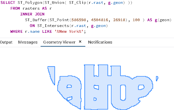
ST_Polygon considers all the pixels that have values (not no-data) in a particular band, and converts them to geometry. Like many other functions in raster, ST_Polygon only considers 1 band. If no band is specified, it will consider only the first band.
30.6.2. The pixel rectangles of a raster with ST_PixelAsPolygons
Another popularly used function is the ST_PixelAsPolygons function. You should rarely use ST_PixelAsPolygons on a large raster without first clipping because you will end up with millions of rows, one for each pixel.
ST_PixelAsPolygons returns a table consisting of geom, val, x, and y. Where x is the column number, and y is the row number in the raster.
ST_PixelAsPolygons similar to other raster functions works on one band at a time and works on band 1 if no band is specified. It also by default returns only pixels that have values.
SELECT gv.*
  FROM rasters AS r
    CROSS JOIN LATERAL ST_PixelAsPolygons(rast) AS gv
  WHERE r.name LIKE '%New York%'
  LIMIT 10;
Which outputs:
and if we inspect using the geometry viewer, we’d see:
If we want all pixels of all our bands, we’d need to do something like below. Note the differences in this example from previous.
1. Setting exclude_nodata_value to make sure all pixels are returned so that our sets of calls return the same number of rows. The rows out of the function will be naturally in the same order.
2. Using the PostgreSQL ROWS FROM constructor , and aliasing each set of columns from our function output with names. So for example the band 1 columns (geom, val, x, y) are renamed to g1, v1, x1, x2
SELECT pp.g1, pp.v1, pp.v2, pp.v3
  FROM rasters AS r
    CROSS JOIN LATERAL
    ROWS FROM (
      ST_PixelAsPolygons(rast, 1, exclude_nodata_value => false ),
      ST_PixelAsPolygons(rast, 2, exclude_nodata_value => false),
      ST_PixelAsPolygons(rast, 3, exclude_nodata_value => false )
      ) AS pp(g1, v1, x1, y1,
        g2, v2, x2, y2,
        g3, v3, x3, y3 )
  WHERE r.name LIKE '%New York%'
   AND ( pp.v1 = 0 OR  pp.v2 > 0 OR pp.v3 > 0) ;
Note
We used CROSS JOIN LATERAL in these examples because we wanted to be explicit what we are doing. Since these are all set returning functions, you can replace CROSS JOIN LATERAL with , for short-hand. We’ll use a , in the next set of examples
30.6.3. Dumping polygons with ST_DumpAsPolygons
Raster also introduces an additional composite type called a geomval. Consider a geomval as the offspring of a geometry and raster. It contains a geometry and it contains a pixel value.
You will find several raster functions that return geomvals.
A commonly used function that outputs geomvals is ST_DumpAsPolygons, which returns a set of contiguous pixels with the same value as a polygon. Again this by default will only check band 1 and exclude no data values unless you override. This example selects only polygons from band 2. You can also apply filters to the values. For most use cases, ST_DumpAsPolygons is a better option than ST_PixelAsPolygons as it will return far fewer rows.
This will output 6 rows, and return polygons corresponding to the letters in “Raster”.
SELECT gv.geom , gv.val
  FROM rasters AS r,
    ST_DumpAsPolygons(rast, 2) AS gv
  WHERE r.name LIKE '%New York%'
      AND gv.val = 100;
Note that it doesn’t return a single geometry, because it finds continguous set of pixels with the same value that form a polygon. Even though all these values are the same, they are not continguous.

A common approach to produce more complex geometries is to group by the values and union.
SELECT ST_Union(gv.geom) AS geom , gv.val
  FROM rasters AS r,
    ST_DumpAsPolygons(rast, 2) AS gv
  WHERE r.name LIKE '%New York%'
  GROUP BY gv.val;
This will give you 2 rows back corresponding to the words “Raster” and “Hello”.
30.7. Statistics
The most important thing to understand about rasters is that they are statistical tools for storing data in arrays, that you may happen to be able to make look pretty on a screen.
You can find a menu of these statistical functions in Raster Band Statistics.
30.7.1. ST_SummaryStatsAgg and ST_SummaryStats
Want all stats for a set or rasters, reach for the function ST_SummaryStatsAgg.
This query takes about 10 seconds and gives you a summary of the whole table:
SELECT (ST_SummaryStatsAgg(rast, 1, true, 1)).* AS sa
    FROM o_3_nyc_dem;
Outputs:
count      |    sum     |       mean       |      stddev      | min | max
-----------+------------+------------------+------------------+-----+-----
246794100  | 4555256024 | 18.4577184948911 | 39.4416860598687 |   0 | 411
(1 row)
Which tells we have a lot of pixels and our max elevation is 411 ft.
If you have built overviews, and just need a rough estimate of your mins, maxs, and means use one of your overviews. This next query returns roughly the same values for mins, maxs, and means as the prior but in about 1 second instead of 10.
SELECT (ST_SummaryStatsAgg(rast, 1, true, 1)).* AS sa
    FROM o_3_nyc_dem ;
Now armed with this bit of information, we can ask more questions.
30.7.2. ST_Histogram
Generally you won’t want stats for your whole table, but instead just stats for a particular area, in that case, you’ll want to also employ our old friends ST_Intersects and ST_Clip. If you are also in need of a raster statistics function that doesn’t have an aggregate version, you’ll want to carry ST_Union along for the ride.
For this next example we’ll use a different stats function ST_Histogram which has no aggregate equivalent, and for this particular variant, is a set returning function. We are using the same area of interest as some prior examples, but we also need to employ geometry ST_Transform to transform our NY state plane meters geometry to our NYC State Plane feet rasters. It is almost always more performant to transform the geometry instead of raster and definitely if your geometry is just a single one.
SELECT (ST_Quantile( ST_Union( ST_Clip(r.rast, g.geom) ), ARRAY[0.25,0.50,0.75, 1.0] )).*
    FROM nyc_dem AS r
       INNER JOIN
        ST_Transform(
          ST_Buffer(ST_Point(586598, 4504816, 26918), 100 ),
            2263) AS g(geom)
        ON  ST_Intersects(r.rast, g.geom);
the above query completes in under 60ms and outputs:
quantile  | value
----------+-------
    0.25  |    52
    0.5   |    57
    0.75  |    68
    1     |    78
(4 rows)
30.8. Creating Derivative Rasters
PostGIS raster comes packaged with a number of functions for editing rasters. These functions are both used for editing as well as creating derivative raster data sets. You will find these listed in Raster Editors and Raster Management.
30.8.1. Transforming rasters with ST_Transform
Most of our data is in NY State Plane meters (SRID: 26918), however our DEM raster dataset is in NY State Plane feet (SRID: 2263). For the least cumbersome workflow, we need our core datasets to be in the same spatial reference system.
The raster ST_Transform is the function most suited for this job.
In order to create a new nyc dem dataset in NY State Plane meters, we’ll do the following:
CREATE TABLE nyc_dem_26918 AS
WITH ref AS (SELECT ST_Transform(rast,26918) AS rast
            FROM nyc_dem LIMIT 1)
SELECT r.rid, ST_Transform(r.rast, ref.rast) AS rast, r.filename
FROM nyc_dem AS r, ref;
The above on my system took about 1.5 minutes. For a larger data set it would take much longer.
The aforementioned examples used two variants of the ST_Transform raster function. The first was to get a reference raster that will be used to transform the other raster tiles to guarantee that all tiles have the same alignment. Note the second variant of ST_Transform used doesn’t even take an input SRID. This is because the SRID and all the pixel scale and block sizes are read from the reference raster. If you used ST_Transform(rast, srid) form, then all your rasters might come out with different alignment making it impossible to apply an operation such as ST_Union on them.
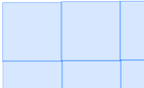
The only problem with the aforementioned ST_Transform approach is that when you transform, the transformed often exists in other tiles. If you looked at the above output closely enough by outputting the convex hull of the rasters, in the next example you’d see annoying overlaps around the borders.
SELECT rast::geometry
  FROM nyc_dem_26918
  ORDER BY rid
LIMIT 100;
viewed in pgAdmin would look something like:
30.8.2. Using ST_MakeEmptyCoverage to create even tiled rasters
A better approach, albeit a bit slower, is to define your own coverage tile structure from scratch using ST_MakeEmptyCoverage and then find the intersecting tiles for each new tile, and ST_Union these and then use ST_Transform(ref, ST_Union…) to create each tile.
For this we’ll be using quite a few functions, we learned about earlier.
DROP TABLE IF EXISTS nyc_dem_26918;
CREATE TABLE nyc_dem_26918 AS
SELECT ROW_NUMBER() OVER(ORDER BY t.rast::geometry) AS rid,
  ST_Union(ST_Clip( ST_Transform( r.rast, t.rast, 'Bilinear' ), t.rast::geometry ), 'MAX') AS rast
FROM (SELECT ST_Transform(
    ST_SetSRID(ST_Extent(rast::geometry),2263)
        , 26918) AS geom
      FROM nyc_dem
    ) AS g, ST_MakeEmptyCoverage(tilewidth => 256, tileheight => 256,
                  width => (ST_XMax(g.geom) - ST_XMin(g.geom))::integer,
                  height => (ST_YMax(g.geom) - ST_YMin(g.geom))::integer,
                  upperleftx => ST_XMin(g.geom),
                  upperlefty => ST_YMax(g.geom),
                  scalex =>  3.048,
                  scaley => -3.048,
                  skewx => 0., skewy => 0., srid => 26918) AS t(rast)
          INNER JOIN nyc_dem AS r
            ON ST_Transform(t.rast::geometry, 2263) && r.rast
GROUP BY t.rast;
Repeating the same exercise as earlier:
SELECT rast::geometry
  FROM nyc_dem_26918
  ORDER BY rid
LIMIT 100;
viewed in pgAdmin we no longer have overlaps:

On my system this took ~10 minutes and returned 3879 rows. After the creation of the table, we’ll want to do the usual of adding a spatial index, primary key, and constraints as follows:
ALTER TABLE nyc_dem_26918
  ADD CONSTRAINT pk_nyc_dem_26918 PRIMARY KEY(rid);

CREATE INDEX ix_nyc_dem_26918_st_convexhull_gist
    ON nyc_dem_26918 USING gist( ST_ConvexHull(rast) );

SELECT AddRasterConstraints('nyc_dem_26918'::name, 'rast'::name);
ANALYZE nyc_dem_26918;
Which should take under 2 minutes for this dataset.
30.8.3. Creating overview tables with ST_CreateOverview
Just as with our original dataset, it would be useful to have overview tables to speed up performance of some operations. ST_CreateOverview is a function fit for that purpose. You can use ST_CreateOverview to create overviews also if you neglected to create one during the raster2pgsql load or you decided, you need more overviews.
We’ll create level 2 and 3 overviews as we had done with our original using this code.
SELECT ST_CreateOverview('nyc_dem_26918'::regclass, 'rast', 2);
SELECT ST_CreateOverview('nyc_dem_26918'::regclass, 'rast', 3);
This process sadly takes a while, and a longer while the more rows you have so be patient. For this dataset it took about 3-5 minutes for the overview factor 2 and 1 minute for the overview factor 3.
The ST_CreateOverView function also adds in the needed constraints so the columns appear with full detail in the raster_columns and raster_overviews catalogs. It does not add indexes to them though and also does not add an rid column. The rid column is probably not necessary unless you need a primary key to edit with. You would probably want an index which you can create with the following:
CREATE INDEX ix_o_2_nyc_dem_26918_st_convexhull_gist
    ON o_2_nyc_dem_26918 USING gist( ST_ConvexHull(rast) );

CREATE INDEX ix_o_3_nyc_dem_26918_st_convexhull_gist
    ON o_3_nyc_dem_26918 USING gist( ST_ConvexHull(rast) );
Note
ST_CreateOverview has an optional argument for denoting the sampling method. If not specified it uses the default NearestNeighbor which is generally the fastest to compute but may not be ideal. Resampling methods is beyond the scope of this workshop.
30.9. The intersection of rasters and geometries
There are a couple of functions commonly used to compute intersections of rasters and geometries. We’ve already seen ST_Clip in action which returns the intersection of a raster and geometry as a raster, but there are others. For point data, the most commonly used is ST_Value and then there is the ST_Intersection which has several overloads some returning rasters and some returning a set of geomval.
30.9.1. Pixel values at a geometric Point
If you need to return values from rasters based on intersection of several ad-hoc geometry points, you’ll use ST_Value or it’s nearest relative ST_NearestValue.
SELECT g.geom, ST_Value(r.rast, g.geom) AS elev
  FROM nyc_dem_26918 AS r
    INNER JOIN
    (SELECT id, geom
      FROM nyc_homicides
      WHERE weapon = 'gun') AS g
      ON r.rast && g.geom;
This example takes about 1 second to return 2444 rows. If you used ST_Intersects instead of &&, the process would take about 3 seconds. The reason ST_Intersects is slower is that it performs an additional recheck in some cases a pixel by pixel check. If you expect all your points to be represented with data in your raster set and your rasters represent a coverage (a continguous set non-overlapping raster tiles), then && is generally a speedier option.
If your raster data is not densely populated or you have overlapping rasters (e.g. they represent different observations in time), or they are skewed (not axis aligned) then there is an advantage to having ST_Intersects weed out the false positives.
30.9.2. ST_Intersection raster style
Just as you can compute the intersection of two geometries using ST_Intersection, you can compute intersection of two rasters or a raster and a geometry using raster ST_Intersection.
What you get out of this beast, are two different kinds of things:
Intersect a geometry with a raster, and you get a set of geomval offspring. Perhaps one, but most often many.
Intersect 2 rasters and you get a single raster back.
The golden rule for both raster intersection and geometry intersection is that both parties involved must have the same spatial reference system. For raster/raster, they also have to have same alignment.
Here is an example which answers a question you may have been curious about. If we bucket our elevations into 5 buckets of elevation values, which elevation range results in the most gun fatalities? We know based on our earlier summary statistics that 0 is the lowest value and 411 is the highest value for elevation in our nyc dem dataset, so we use that as min and max value for our width_bucket call.
SELECT ST_Transform(ST_Union(gv.geom),4326) AS geom ,
  MIN(gv.val) AS min_elev, MAX(gv.val) AS max_elev,
    count(g.id) AS count_guns
  FROM nyc_dem_26918 AS r
    INNER JOIN nyc_homicides AS g
      ON ST_Intersects(r.rast, g.geom)
    CROSS JOIN
     ST_Intersection( g.geom,
      ST_Clip(r.rast,ST_Expand(g.geom, 4) )
      ) AS gv
  WHERE g.weapon = 'gun'
  GROUP BY width_bucket(gv.val, 0, 411, 5)
  ORDER BY width_bucket(gv.val, 0, 411, 5);
Is there an important correlation between gun homicides and elevation? Probably not.
Let’s take a look at raster / raster intersection:
SELECT ST_Intersection(r1.rast, 1, r2.rast, 1, 'BAND1')
  FROM nyc_dem_26918 AS r1
    INNER JOIN
        rasters AS r2 ON ST_Intersects(r1.rast,1, r2.rast, 1);
What we get are two rows with NULLLs, and if you have your PostgreSQL set to show notices, you’ll see:
NOTICE: The two rasters provided do not have the same alignment. Returning NULL
In order to fix this, we can align one to the other as it’s coming out of the gate using ST_Resample.
SELECT ST_Intersection(r1.rast, 1,
  ST_Resample( r2.rast, r1.rast ), 1,
    'BAND1')
  FROM nyc_dem_26918 AS r1
    INNER JOIN
        rasters AS r2 ON ST_Intersects(r1.rast,1, r2.rast, 1);
Let’s also roll it up into a single stats record
SELECT (
  ST_SummaryStatsAgg(
    ST_Intersection(r1.rast, 1,
      ST_Resample( r2.rast, r1.rast ), 1, 'BAND1'),
        1, true)
    ).*
  FROM nyc_dem_26918 AS r1
    INNER JOIN
        rasters AS r2 ON ST_Intersects(r1.rast,1, r2.rast, 1);
which outputs:
count  |  sum  |      mean       |      stddev      | min | max
-------+-------+-----------------+------------------+-----+-----
  2075 | 99536 | 47.969156626506 | 9.57974836865737 |  33 |  62
(1 row)
30.10. Map Algebra Functions
Map algebra is the idea that you can do math on your pixel values. The ST_Union and ST_Intersection functions covered earlier are a special fast case of map algebra. Then there are the ST_MapAlgebra family of functions which allow you to define your own crazy math, but at cost of performance.
People have the habit of jumping to ST_MapAlgebra, probably because the name sounds so cool and sophisticated. Who wouldn’t want to tell their friends? I’m using a function called ST_MapAlgebra. My advice, explore other functions before you pull out that shotgun. Your life will be simpler and your performance will be 100 times better, and your code will be shorter.
Before we showcase ST_MapAlgebra, we’ll explore other functions that fit under the Map Algebra family of functions and generally have better performance than ST_MapAlgebra.
30.10.1. Reclassify your raster using ST_Reclass
An often overlooked map-algebraish function is the ST_Reclass function, who sits in the background waiting for someone to discover the power and speed it can offer.
What does ST_Reclass do? It as the name implies, reclassifies your pixel values based on minimalist range algebra.
Lets revisit our NYC Dems. Perhaps we only care about classifying our elevations as 1) low, 2) medium, 3) high , and 4) really high. We don’t need 411 values, we just need 4. With that said lets do some reclassifying.
The classification scheme is governed by the reclass expression.
WITH r AS ( SELECT ST_Union(newrast) As rast
  FROM nyc_dem_26918 AS r
        INNER JOIN ST_Buffer(ST_Point(586598, 4504816, 26918), 1000 ) AS g(geom)
          ON ST_Intersects( r.rast, g.geom )
        CROSS JOIN ST_Reclass( ST_Clip(r.rast,g.geom), 1,
          '[0-10):1, [10-50):2, [50-100):3,[100-:4','4BUI',0) AS newrast
        )
SELECT SUM(ST_Area(gv.geom)::numeric(10,2)) AS area, gv.val
    FROM r, ST_DumpAsPolygons(rast) AS gv
    GROUP BY gv.val
    ORDER BY gv.val;
Which would output:
  area      | val
------------+-----
    6754.04 |   1
1753117.51  |   2
1355232.37  |   3
    1848.75 |   4
(4 rows)
If this were a classification scheme we preferred, we could create a new table using the ST_Reclass to recompute each tile.
30.10.2. Coloring your rasters with ST_ColorMap
The ST_ColorMap function is another mapalgebraish function that reclassifies your pixel values. Except it is band creating. It converts a single band raster such as our Dems into a visually presentable 3 or 4 banded raster.
You could use one of the built-in colormaps as below if you don’t want to fuss with creating one.
SELECT ST_ColorMap( ST_Union(newrast), 'bluered') As rast
   FROM nyc_dem_26918 AS r
       INNER JOIN
         ST_Buffer(
           ST_Point(586598, 4504816, 26918), 1000
           ) AS g(geom)
       ON ST_Intersects( r.rast, g.geom)
        CROSS JOIN ST_Clip(rast, g.geom) AS newrast;
Which looks like:
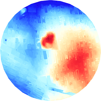
The bluer the color the lower the elevation and the redder the color the higher the elevation.
